Sarvasの式3

Sarvasの式で、球の中心を動かしてみます。
電流の位置を(7,0,0)cm、大きさを(0,0,20)nAとして中心(0,0,0)cm、半径12cmの球面上のセンサーでの磁場を計算しますが、 均質導体モデルの球の中心座標をいろいろ変化させてみます。

getf('../Sarvas.sce');
stacksize(50000000);
t=linspace(-%pi,%pi,37)';
p=linspace(-%pi/2,%pi/2,19);
r=0.12;
x=r*cos(t)*cos(p);
y=r*sin(t)*cos(p);
z=r*ones(t)*sin(p);
[xx,yy,zz]=nf3d(x,y,z);
xx=xx($:-1:1,:);yy=yy($:-1:1,:);zz=zz($:-1:1,:);
scale=64/2;
scf();set(gcf(),'color_map',jetcolormap(scale*2));
q=[0.07,0,0,0,0,20*1e-9];
kr=size(x,1);kc=size(x,2);
x=matrix(x,kr*kc,1);
y=matrix(y,kr*kc,1);
z=matrix(z,kr*kc,1);
R=[x,y,z];

//// ルーチンタスクを関数化 ////
function ShowSarvas(Bz,scale,kr,kc);
Bzc=(Bz*1e+15)/250*scale+scale;
scale2=scale*2;
Bzc(Bzc>scale2)=scale2;Bzc(Bzc<1)=1;
Bzc=matrix(Bzc,kr,kc);
krkc=(kr-1)*(kc-1);
Bzcc=[...
matrix(Bzc(1:($-1),1:($-1)),1,krkc);...
matrix(Bzc(2:$,1:($-1)),1,krkc);...
matrix(Bzc(2:$,2:$),1,krkc);...
matrix(Bzc(1:($-1),2:$),1,krkc)];
Bzcc=Bzcc($:-1:1,:);
hf=gcf();hf.visible='off';
ha=gca();f=ha.children.data;
TL=tlist(['3d','x','y','z','color'],f.x,f.y,f.z,Bzcc);
ha.children.data=TL;
ha.children.color_mode=-1;
ha.children.color_flag=3;
ha.isoview='on';ha.box='off';
ha.rotation_angles=[90,0];
ha.margins=[0,0,0,0];
//ha.tight_limits='on';//何故か強制終了
hf.visible='on';
endfunction;

//// Draw Process ////
subplot(231);plot3d(xx,yy,zz)
Bz=sum(Sarvas(q,R,[0,0,0]).*R/r,2);//(0,0,0)cm
ShowSarvas(Bz,scale,kr,kc);
subplot(234);plot3d(xx,yy,zz)
Bz=sum(Sarvas(q,R,[-0.04,0,0]).*R/r,2);//(4,0,0)cm
ShowSarvas(Bz,scale,kr,kc);
subplot(232);plot3d(xx,yy,zz)
Bz=sum(Sarvas(q,R,[0,0.04,0]).*R/r,2);//(0,4,0)cm
ShowSarvas(Bz,scale,kr,kc);
subplot(233);plot3d(xx,yy,zz)
Bz=sum(Sarvas(q,R,[0,0,0.04]).*R/r,2);//(0,0,4)cm
ShowSarvas(Bz,scale,kr,kc);
subplot(235);plot3d(xx,yy,zz)
Bz=sum(Sarvas(q,R,[0,-0.04,0]).*R/r,2);//(0,-4,0)cm
ShowSarvas(Bz,scale,kr,kc);
subplot(236);plot3d(xx,yy,zz)
Bz=sum(Sarvas(q,R,[0,0,-0.04]).*R/r,2);//(0,0,-4)cm
ShowSarvas(Bz,scale,kr,kc);

球モデルの中心座標の位置による等磁界線図の変化

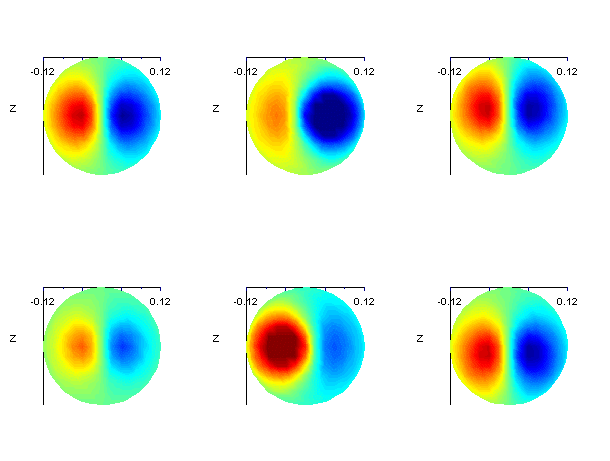
左上は(0,0,0)cmです。Biot-Sarvartと同じです。
左下は(4,0,0)cmです。
中上は(0,4,0)cm、中下は(0,-4,0)cm、
右上は(0,0,4)cm、右下は(0,0,-4)cmです。
Biot-Savartの式では全く関係ありませんが、導体球モデルの位置により、等磁界線図が変化することがわかりました。