加算波形の三次元表示
Python 2.7です。
import sys
print(sys.version_info)
del sys
データの読み込み
import mne
mne.set_log_level('INFO')
# filename='H:\\FS\\hashizume_akira\\041029\\SEF_median_ave.fif'
filename='c:\\170207\\hashizume_akira\\041029\\SEF_median_ave.fif'
meg=mne.read_evokeds(filename,proj=True)[0] # リストですけど1個しかありません
print(meg)
# 脳磁図波形の前処置
tmin,tmax=-0.05,0.1
def showwave(meg,tmin,tmax):
    meg.copy().crop(tmin=tmin,tmax=tmax).plot();

# 元波形
showwave(meg,tmin,tmax)

# 基線補正
meg.apply_baseline(baseline=(None,0))
showwave(meg,tmin,tmax)

# 2~100Hzの周波数フィルタ
x=meg.data
Fs=meg.info['sfreq']
mne.filter.band_pass_filter(x=x,Fs=Fs,Fp1=2,Fp2=100)
showwave(meg,tmin,tmax)


MNE-Cで以下のコマンドを入力します。
cd subject
mne_wathershed_bem --atlas
cd ./bem/watershed
mne_convert_surface --surf inner_skull_surface --surfout ../inner_skull.surf
mne_convert_surface --surf outer_skull_surface --surfout ../outer_skull.surf
mne_convert_surface --surf outer_skin_surface --surfout ../outer_skuk.surf
# FreeSurferで切り出して作成したメッシュの確認
# subjects_dir='H:\\FS'
subjects_dir='c:\\170207'
subject='hashizume_akira'
mne.viz.plot_bem(subject=subject,subjects_dir=subjects_dir,brain_surfaces='white',orientation='coronal');

# センサと頭皮の座標合わせ
# mne_analyzeなどで座標合わせしてください
trans=subjects_dir+'\\'+subject+'\\041029\\041029-trans.fif'
# jupyterではうまく描画できません
# mne.viz.plot_trans(meg.info,trans,subject=subject,dig=True,meg_sensors=True,subjects_dir=subjects_dir);
python consoleでは以下の図が描画されます。
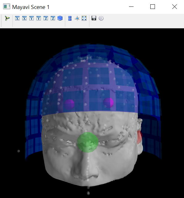
python console用です。
import mne
filename='c:\\170207\\hashizume_akira\\041029\\SEF_median_ave.fif'
trans=subjects_dir+'\\'+subject+'\\041029\\041029-trans.fif'
meg=mne.read_evokeds(filename,proj=True)[0]
subjects_dir='c:\\170207'
subject='hashizume_akira'
mne.viz.plot_trans(meg.info,trans,subject=subject,dig=True,meg_sensors=True,subjects_dir=subjects_dir);
# 格子点の設定
src=mne.setup_source_space(subject,spacing='oct6',subjects_dir=subjects_dir,add_dist=False,overwrite=True)
print(src)
クラスSourceSpace srcを細かく見てみます。
print('src list: %d' %len(src))
print(src[0].keys())
print('nearest, dist, dist, dist_limit, pinfo, nearest_dist, patch_inds: None') # NoneType
print('nn: %d x %d' %src[0]['nn'].shape+ ' + %d x %d' %src[1]['nn'].shape)
print('rr: %d x %d' %src[0]['rr'].shape+ '+ %d x %d' %src[1]['rr'].shape)
print('inuse: %d' %src[0]['inuse'].shape+' + %d' %src[1]['inuse'].shape)
print('nuse: %d' %src[0]['nuse']+ ' + %d' %src[1]['nuse'])
print('vertno: %d' %len(src[0]['vertno'])+' + %d' %len(src[1]['vertno']))
print('nuse_tri: %d' %src[0]['nuse_tri']+' + %d' %src[1]['nuse_tri'])
print('coord_frame: %d' %src[0]['coord_frame'])
print('ntri: %d' %src[0]['ntri']+' + %d' %src[1]['ntri'])
print('np: %d' %src[0]['np']+' + %d' %src[1]['np'])
print('subject_his_id: '+src[0]['subject_his_id'])
print('use_tris: %d x %d' %src[0]['use_tris'].shape)
print('type: '+src[0]['type']+' + '+src[1]['type'])
print('id: %d + %d' %(src[0]['id'], src[1]['id']))
print('tris: %d x %d' %src[0]['tris'].shape +' + %d x %d' %src[1]['tris'].shape)
srcは本来
mne.write_source_spaces(subject-oct-6-src.fif)
で保存するですが、上mne.setup_source_spaceを実行するとsubject-oct-6-src.fifという名前で保存されています。
del(src)
# srcの読み込み
src_name=subjects_dir+'\\'+subject+'\\bem\\'+subject+'-oct-6-src.fif'
src=mne.read_source_spaces(src_name);
print(src)
# 格子点の確認
mne.viz.plot_bem(subject=subject,subjects_dir=subjects_dir,brain_surfaces='white',src=src,orientation='coronal');

# jupyterではうまく描画されません
import numpy as np
from mayavi import mlab
from surfer import Brain
#brain=Brain('hashizume_akira','lh','inflated',subjects_dir=subjects_dir);
#surf=brain._geo
vertidx=np.where(src[0]['inuse'])[0]
#mlab.points3d(surf.x[vertidx],surf.y[vertidx],surf.z[vertidx],color=(1,1,0),scale_factor=1.5);
python consoleでは以下の図になります。
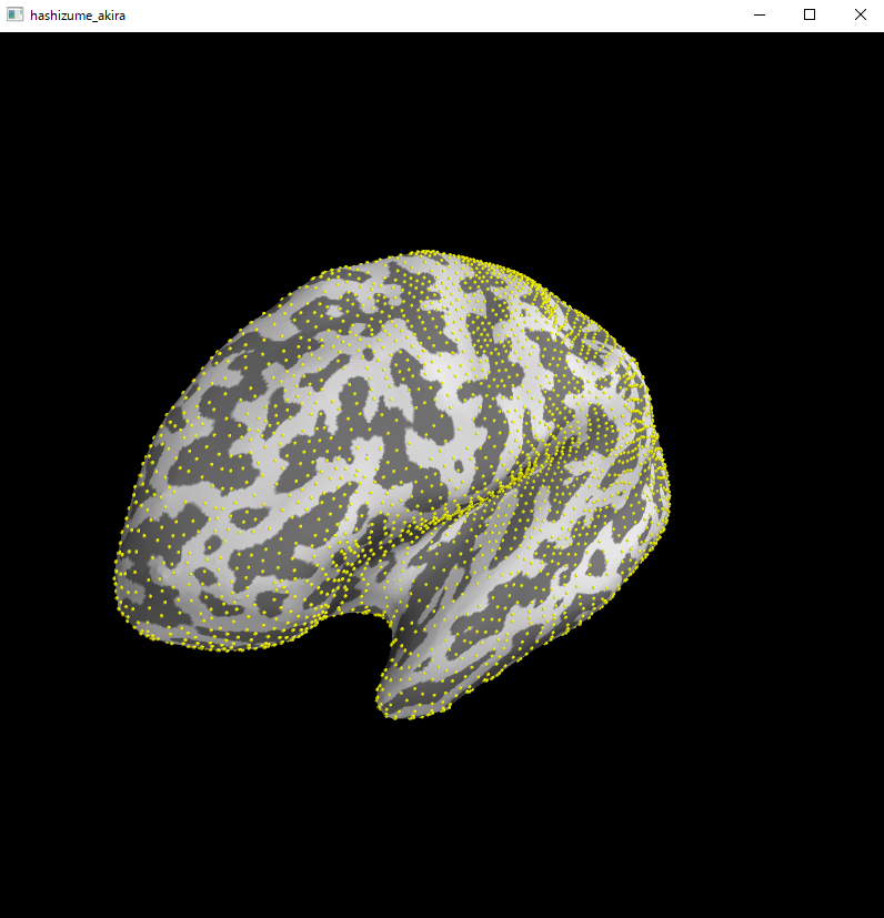
python console用です
import numpy as np
from mayavi import mlab
from surfer import Brain
import mne
subject='hashizume_akira'
subjects_dir='c:\\170207'
brain=Brain(subject,'lh','inflated',subjects_dir=subjects_dir);
surf=brain._geo
src_name=subjects_dir+'\\'+subject+'\\bem\\'+subject+'-oct-6-src.fif'
src=mne.read_source_spaces(src_name);
vertidx=np.where(src[0]['inuse'])[0]
mlab.points3d(surf.x[vertidx],surf.y[vertidx],surf.z[vertidx],color=(1,1,0),scale_factor=1.5);
conductivity=(0.3,) # single layer
model=mne.make_bem_model(subject='hashizume_akira',ico=4,conductivity=conductivity,subjects_dir=subjects_dir)
print('model list: %d' %len(model))
print(model[0].keys())
print('nn: %d x %d' %model[0]['nn'].shape)
print('rr: %d x %d' %model[0]['rr'].shape)
print('coord_frame: %d' %model[0]['coord_frame'])
print('ntri: %d' %model[0]['ntri'])
print('np: %d' %model[0]['np'])
print('sigma: %0.2f' %model[0]['sigma'])
print('id: %d' %model[0]['id'])
print('tris: %d x %d' %model[0]['tris'].shape)
BEM surfaceのファイルの読み書きは以下の通りです
ntri=model[0]['ntri']
surface_fname=subject+'-%d-%d-%d-bem.fif' %(ntri, ntri, ntri)
mne.write_bem_surfaces(surface_fname,model)
del model
model=mne.read_bem_surfaces(surface_fname)
print('ntri: %d' %model[0]['ntri'])
bem=mne.make_bem_solution(model)
print(bem)
クラスConductorModelのbemの中身を見てみます。
print(bem.keys())
print('nsol: %d' %bem['nsol'])
print('field_mult: %0.9f' %bem['field_mult'])
print('solution: %d x %d' %bem['solution'].shape)
print('is_sphere: False') #bem['is_sphere]
print('bem_method: %d' %bem['bem_method'])
print('soruce_mult: %0.9f' %bem['source_mult'])
print('sigma: %0.9f' %bem['sigma'])
print('gamma: %0.9f' %bem['gamma'])
print('surf list: %d' %len(bem['surfs']))
print(bem['surfs'][0].keys())
print('surf nn: %d x %d' %bem['surfs'][0]['nn'].shape)
print('surf rr: %d x %d' %bem['surfs'][0]['rr'].shape)
print('surf tri_cent: %d x %d' %bem['surfs'][0]['tri_cent'].shape)
print('surf neighbor_tri (list): %d' %len(bem['surfs'][0]['neighbor_tri']))
print('surf neighbor_tri[0] : %d' %len(bem['surfs'][0]['neighbor_tri'][0]))
print('surf tri_nn: %d x %d' %bem['surfs'][0]['tri_nn'].shape)
print('surf coord_frame: %d' %bem['surfs'][0]['coord_frame'])
print('surf ntri: %d' %bem['surfs'][0]['ntri'])
print('surf np: %d' %bem['surfs'][0]['np'])
print('surf sigma: %0.9f' %bem['surfs'][0]['sigma'])
print('surf id: %d' %bem['surfs'][0]['id'])
print('surf tris: %d x %d' %bem['surfs'][0]['tris'].shape)
print('surf tri_area: %d' %bem['surfs'][0]['tri_area'].shape)
modelの辞書にtri_cent, neighbor_tri, tri_nn, tri_areaが追加され、bemにsurfsという項目で追加されます。
クラスConductorModelのファイルの読み書きは以下の通りです。
ntri=bem['surfs'][0]['ntri']
bem_fname=subjects_dir+'\\'+subject+'\\bem\\'+subject+'-%d-%d-%d-bem-sol.fif' %(ntri,ntri,ntri)
mne.write_bem_solution(bem_fname,bem)
del bem
bem=mne.read_bem_solution(bem_fname)
# 磁場計算行列 Lead field matrix の計算
# megでなくmeg.infoです
fwd=mne.make_forward_solution(meg.info,trans=trans,src=src,bem=bem,fname=None,meg=True,eeg=False,mindist=5.0,n_jobs=3)
# fwdの中身
print(fwd)
print(fwd.keys())
print(fwd['info'])
print('sol_grad: None') #fwd['sol_grad'])
print('nchan: %d' %fwd['nchan'])
print('src: src') # print(fwd['src'])
print('source_nn: %d x %d' %fwd['source_nn'].shape)
print(fwd['sol'].keys())
print('sol row_names: %d' %len(fwd['sol']['row_names']))
print('sol ncol: %d' %fwd['sol']['ncol'])
print('sol data: %d x %d' %fwd['sol']['data'].shape)
print('sol col_names: []') #fwd['sol']['col_names']
print('sol nrow: %d' %fwd['sol']['nrow'])
print('source_rr: %d x %d' %fwd['source_rr'].shape)
print('_orig_sol_grad: None') #fwd['_orig_sol_grad'])
print('surf_ori: False') #fwd['surf_ori'])
print('coord_frame: %d' %fwd['coord_frame'])
print('source_ori: %d' %fwd['source_ori'])
print('_orig_sol: %d x %d' %fwd['_orig_sol'].shape)
print('mri_head_t: MRI (surface RAS)->head') #fwd['mri_head_t']
print('nsource: %d' %fwd['nsource'])
print('_orig_source_ori: %d' %fwd['_orig_source_ori'])
Lead Field行列はfwd['sol']['data']です。
クラスForward fwdのファイルの読み書きは以下の通りです。
なお、フォルダをbemから脳磁図データのあるフォルダに変更しています。
fwd_fname=subjects_dir+'\\'+subject+'\\041029\\'+subject+'fwd'
mne.write_forward_solution(fwd_fname,fwd,overwrite=True)
del fwd
fwd=mne.read_forward_solution(fwd_fname)
print(fwd)
定常状態の分散行列の作成にはRawやEpochが必要で、Evokedからは作れません。
そこでまずEvokedをRawArrayに変換します。次にSTI 001チャンネルにトリガー信号があり、これを利用して分散行列を計算します。その次にnumpy.cov()を使って分散行列を書き換えます。とりあえず計算できればいいということで細かいことは無視します。
# 雑音行列の計算
# RawArrayに変換
raw=mne.io.RawArray(meg.data,meg.info)
# RawArrayから分散行列計算
noise_cov=mne.compute_raw_covariance(raw)
print(noise_cov.keys())
print('cov data: %d x %d' %noise_cov['data'].shape) # covは306x306の行列であることを確認
# -0.05~0.0秒の脳磁図出ただけを取り出す
meg0=meg.copy().pick_types(meg=True).crop(tmin=-0.05,tmax=0.0)

# -0.05~0.0の分散行列の計算
import numpy
cov2=numpy.cov(meg0.data)
print('cov2: %d x %d' %cov2.shape)
# del numpy # 以後module numpyを使わないとき

# 分散行列の書き換え
noise_cov['data']=cov2
# 脳磁図波形と定常状態の関係など
meg.plot_white(noise_cov);
noise_cov.plot(raw.info,proj=True);


クラスCovarianceのnoise_covのファイルの読み書きは以下の通りです。
cov_fname=subjects_dir+'\\'+subject+'\\041029\\'+'SEF_median_ave-cov.fif'
mne.write_cov(cov_fname,noise_cov)
del noise_cov
noise_cov=mne.read_cov(cov_fname)
print('cov data: %d x %d' %noise_cov['data'].shape)
inverse_operator=mne.minimum_norm.make_inverse_operator(meg.info,fwd,noise_cov,loose=0.2,depth=0.8)
# inverse_operatorの中身
print(inverse_operator.keys())
print('nave: %0.9f' %inverse_operator['nave'])
print('methods: %d'%inverse_operator['methods'])
print('eigen_fields: [row_names, ncol, data, nrow, col_names]') #print(inverse_operator['eigen_fields'].keys())
print('eigen_leads_weighted: False') #print(inverse_operator['eigen_leads_weighted'])
print('fmri_prior: None') #print(inverse_operator['fmri_prior'])
print('orient_prior: [dim, kind, bads, projs, diag, nfree, eig, eigvec, data, names]') #print(inverse_operator['orient_prior'].keys())
print('mri_head_t: MRI (surface RAS->head)') #print(inverse_operator['mri_head_t'])
print('sing: %d' %inverse_operator['sing'].shape)
print('noise_cov: class Covariance')#print(inverse_operator['noise_cov'])
print('nsource: %d' %inverse_operator['nsource'])
print('info: class Info')
print('src: class SourceSpaces') #print(inverse_operator['src'])
print('source_cov: [dim, kind, bads, projs, diag, nfree, names, eig, data, eigvec]')# print(inverse_operator['source_cov'])
print('projs: class Projection')#print(inverse_operator['projs'])
print('source_nn: %d x %d' %inverse_operator['source_nn'].shape)
print('depth_prior: [dim, kind, bads, projs, diag, nfree, eig, eigvec, data, names]')#print(inverse_operator['depth_prior'])
print('source_ori: %d' %inverse_operator['source_ori'])
print('coord_frame: %d' %inverse_operator['coord_frame'])
print('units: Am') #print(inverse_operator['units'])
print('eigen_leads: [row_names, ncol, data,col_names, nrow]') #print(inverse_operator['eigen_leads'])
クラスInverseOperator inverse_operatorのファイルの読み書きは以下の通りです。
inverse_operator_fname=subjects_dir+'\\'+subject+'\\041029\\'+subject+'oct-6-inv.fif'
mne.minimum_norm.write_inverse_operator(inverse_operator_fname,inverse_operator)
del inverse_operator
inverse_operator=mne.minimum_norm.read_inverse_operator(inverse_operator_fname)
print(inverse_operator)
method='dSPM'
snr=3.
lambda2=1./snr**2
stc=mne.minimum_norm.apply_inverse(meg,inverse_operator,lambda2,method=method,pick_ori=None)
print(stc)
# stcの中身
# print(dir(stc))
print('data: %d x %d' %stc.data.shape)
print('lh_data: %d x %d' %stc.lh_data.shape)
print('rh_data: %d x %d' %stc.rh_data.shape)
クラスSourceEstimateのファイルの読み書きは以下の通りです。
左右半球脳表別に保存され、ファイル名は-lh.stc、-rh.stcとなります。
尚、mne.write_source_estimateというmethodはありません。
stc_fname=subjects_dir+'\\'+subject+'\\041029\\SEF_median_ave'
# mne.write_source_estimate(stc_fname,stc) # このmethodはない
stc.save(stc_fname)
del stc
stc=mne.read_source_estimate(stc_fname)
print(stc)
# 図示 8187本も書くと大変なので最大値だけ
import numpy
maxdata=numpy.max(stc.data,axis=0)

import matplotlib.pyplot as plt
%matplotlib inline
plt.plot(1e3*stc.times,maxdata);
plt.xlim([-50.,100.]);

10~30 msの最大値の場所・時間を求めます。両側半球で求めることはできません。左半球か、右半球か指定する必要があります。
vertino_max,time_max=stc.get_peak(hemi='lh',tmin=0.01,tmax=0.03)
clim=dict(kind='value',lims=[30,400,500])
# jupyterではうまく描画されず
#brain=stc.plot(subject=subject,surface='inflated',hemi='both',subjects_dir=subjects_dir,clim=clim,initial_time=time_max,time_unit='s');
#brain.add_foci(vertno_max,coords_as_verts=True,hemi='lh',color='blue',scale_factor=0.6);
python consoleでは以下の図となります。
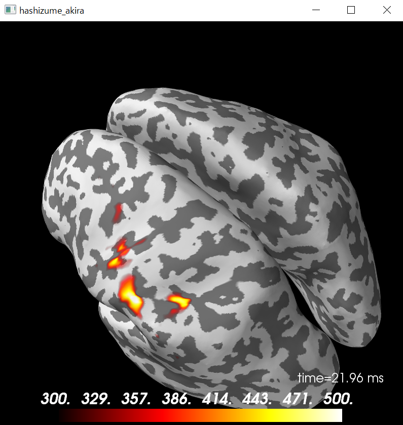
python console用
import mne
subjects_dir='c:\\170207'
subject='hashizume_akira'
stc_fname=subjects_dir+'\\'+subject+'\\041029\\SEF_median_ave'
stc=mne.read_source_estimate(stc_fname)
vertno_max,time_max=stc.get_peak(hemi='lh',tmin=0.01,tmax=0.03)
clim=dict(kind='value',lims=[300,400,500])
brain=stc.plot(subject=subject,surface='inflated',hemi='both',subjects_dir=subjects_dir,clim=clim,initial_time=time_max,time_unit='s');
brain.add_foci(vertno_max,coords_as_verts=True,hemi='lh',color='blue',scale_factor=0.6);
surfaceをinflated以外にしてみました。
# jupyterではうまく描画されず
#brain=stc.plot(subject=subject,surface='white',hemi='both',subjects_dir=subjects_dir,clim=clim,initial_time=time_max,time_unit='s',);
#brain.add_foci(vertno_max,coords_as_verts=True,hemi='lh',color='blue',scale_factor=0.6);
python consoleでは以下の図になります。
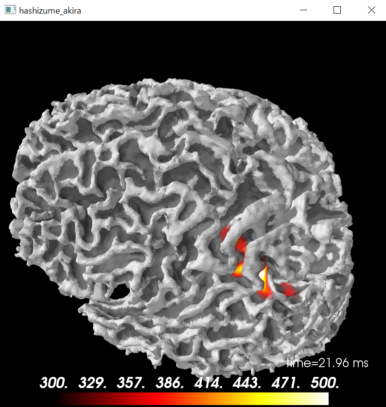
python console用
import mne
subjects_dir='c:\\170207'
subject='hashizume_akira'
stc_fname=subjects_dir+'\\'+subject+'\\041029\\SEF_median_ave'
stc=mne.read_source_estimate(stc_fname)
vertno_max,time_max=stc.get_peak(hemi='lh',tmin=0.01,tmax=0.03)
clim=dict(kind='value',lims=[300,400,500])
brain=stc.plot(subject=subject,surface='white',hemi='both',subjects_dir=subjects_dir,clim=clim,initial_time=time_max,time_unit='s');
brain.add_foci(vertno_max,coords_as_verts=True,hemi='lh',color='blue',scale_factor=0.6);
# 単一電流双極子推定
meg1=meg.copy().pick_types(meg=True,eeg=False).crop(0.02,0.025)
dip=mne.fit_dipole(meg1,noise_cov,bem,trans)
#print(dip)の中身
print('dip list: %d' %len(dip))
print('dip[0] list: %d' %len(dip[0])) # クラスDipole
print('dip[0][0]: [times,pos,amplitude,ori,gof,name]');
#print(dip[0][0].times)
#print(dip[0][0].pos)
#print(dip[0][0].amplitude)
#print(dip[0][0].ori)
#print(dip[0][0].gof)
#print(dip[0][0].name)
print('dip[1]: %d x %d' %dip[1].shape) # ndarray
クラスDipoleのdip[0]のファイルの読み書きは以下の通りです。
dip_fname=subjects_dir+'\\'+subject+'\\041029\\SEF_median_ave.dip'
dip[0].save(dip_fname)
del dip
dip=mne.read_dipole(dip_fname) # dip[0]ではない
print(dip)
dip.plot_amplitudes(color='k');
# dip2=dip.copy().crop(tmin=0.022,tmax=0.024) # cropが無効?
dip[2].plot_locations(trans,subject,subjects_dir,mode='orthoview');


# jupyterでは描画されず
# plot_locations()でsphere
# dip[2].plot_locations(trans,subject,subjects_dir,mode='cone');
python consoleでは以下の図になります。
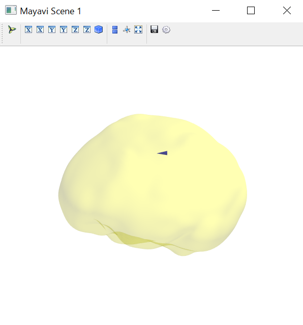
python console用です。
import mne
trans='c:\\170207\\hashizume_akira\\041029\\041029-trans.fif'
subject='hashizume_akira'
subjects_dir='c:\\170207'
dip_fname=subjects_dir+'\\'+subject+'\\041029\\SEF_median_ave.dip'
dip=mne.read_dipole(dip_fname)
dip[2].plot_locations(trans,subject,subjects_dir,mode='cone');