内容
MNE-Pythonのtutorialのこの部分を試してみました。
いろいろ読み込み
いろいろ読み込みます。
import
os.path as op
import
numpy as np
import
matplotlib.pyplot as plt
import
mne
data_path=mne.datasets.sample.data_path()
fname=op.join(data_path,'MEG','sample','sample_audvis-ave.fif')
evoked=mne.read_evokeds(fname,baseline=(None,0),proj=True)
print(evoked)
[<Evoked |
comment : 'Left Auditory', kind :
average,
time : [-0.199795, 0.499488], n_epochs : 55, n_channels x n_times : 376 x 421,
~4.9 MB>,
<Evoked |
comment : 'Right Auditory', kind :
average,
time : [-0.199795, 0.499488], n_epochs : 61, n_channels x n_times : 376 x 421,
~4.9 MB>,
<Evoked |
comment : 'Left visual', kind :
average,
time : [-0.199795, 0.499488], n_epochs : 67, n_channels x n_times : 376 x 421,
~4.9 MB>,
<Evoked |
comment : 'Right visual', kind :
average,
time : [-0.199795, 0.499488], n_epochs : 58, n_channels x n_times : 376 x 421,
~4.9 MB>]
4つの加算波形データがあります。名前を付けておきます。
evoked_l_aud=evoked[0]
evoked_r_aud=evoked[1]
evoked_l_vis=evoked[2]
evoked_r_vis=evoked[3]
波形表示
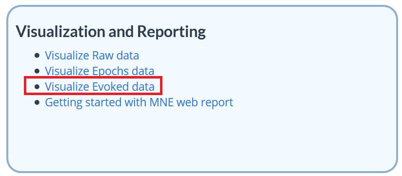
evoked_l_audの波形を表示します。
fig=evoked_l_aud.plot(exclude=())
fig.tight_layout() # グラフを最大化
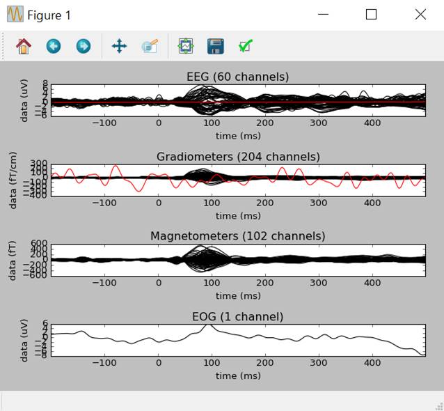
各チャンネルを色別表示します。
picks=mne.pick_types(evoked_l_aud.info,meg=True,eeg=False,eog=False)
evoked_l_aud.plot(spatial_colors=True,gfp=True,picks=picks)
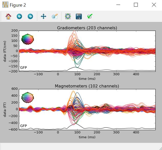
等磁場線図表示
evoked_l_aud.plot_topomap()
初期設定だと10分割のようです。
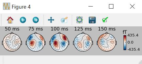
50〜150msまで25msずつの時間帯でmagnetomterだけの等磁場線図を表示します。
times=np.arange(0.05,0.151,0.025) # 25msecずつ
evoked_r_aud.plot_topomap(times=times,ch_type='mag')
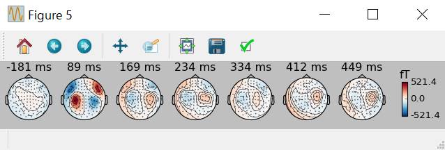
times=’peaks’という引数があると波形の頂点の所を自動的に選んでくれます。
evoked_r_aud.plot_topomap(times='peaks',ch_type='mag')
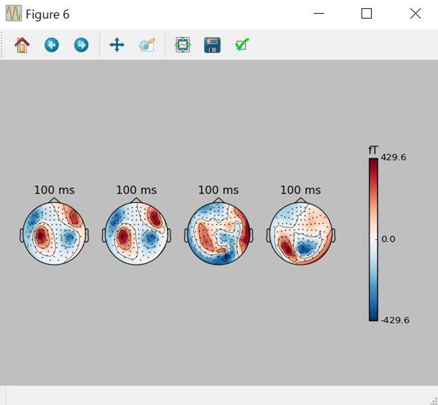
4つの加算平均の100msの等磁場線図を表示します。
fig,ax=plt.subplots(1,5)
evoked_l_aud.plot_topomap(times=0.1,axes=ax[0],show=False)
evoked_r_aud.plot_topomap(times=0.1,axes=ax[1],show=False)
evoked_l_vis.plot_topomap(times=0.1,axes=ax[2],show=False)
evoked_r_vis.plot_topomap(times=0.1,axes=ax[3],show=True)
# colorbarがax[4]
以下の警告が4回出ますが無視します。
<stdin>:1: RuntimeWarning: Colorbar is drawn to the rightmost column of the figure. Be
sure to provide enough space for it or turn it off with colorbar=False.
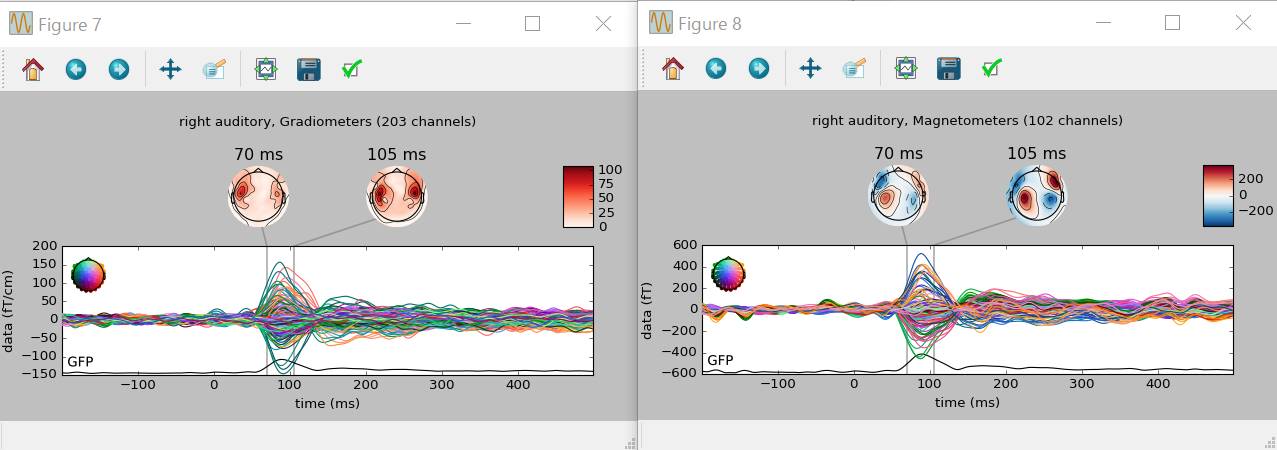
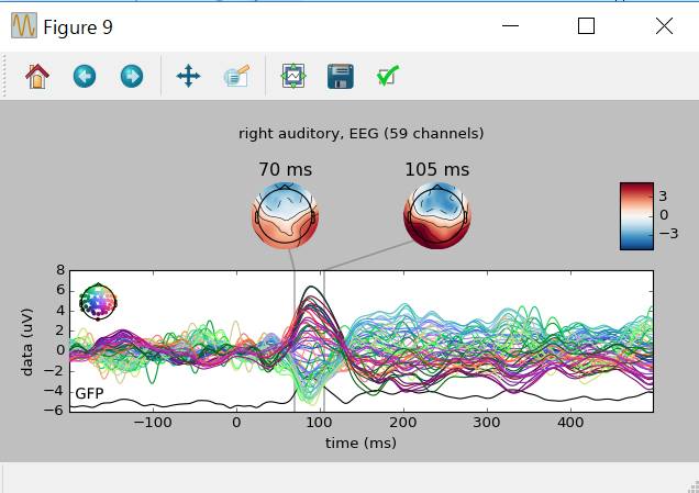
波形と等磁場線図などのトポグラフィを組み合わせます
ts_args=dict(gfp=True)
topomap_args=dict(sensors=False)
evoked_r_aud.plot_joint(title='right
auditory',times=[0.07,0.105],ts_args=ts_args,topomap_args=topomap_args)
左がgradiometer、右がmagnetometerです。
脳波です。
ウインドウを全部閉じます。
plt.close('all')
条件別波形比較
それぞれの条件を読み込みます。
conditions=['Left
Auditory','Right Auditory','Left
visual','Right visual']# Visualでなくvisual
evoked_dict=dict()
for
condition in conditions:
evoked_dict[condition.replace('
','/')]=mne.read_evokeds(fname,baseline=(None,0),proj=True,condition=condition)
print(evoked_dict)
{'Left/Auditory':
<Evoked | comment : 'Left Auditory', kind :
average,
time : [-0.199795, 0.499488], n_epochs : 55, n_channels x n_times : 376 x 421,
~4.9 MB>,
'Right/visual':
<Evoked | comment : 'Right visual', kind :
average,
time : [-0.199795, 0.499488], n_epochs : 58, n_channels x n_times : 376 x 421,
~4.9 MB>,
'Left/visual':
<Evoked | comment : 'Left visual', kind :
average,
time : [-0.199795, 0.499488], n_epochs : 67, n_channels x n_times : 376 x 421,
~4.9 MB>,
'Right/Auditory':
<Evoked | comment : 'Right Auditory', kind :
average,
time : [-0.199795, 0.499488], n_epochs : 61, n_channels x n_times : 376 x 421,
~4.9 MB>}
波形表示させます。
colors=dict(Left='Crimson',Right='CornFlowerBlue')
linestyles=dict(Auditory='-',visual='--')
pick=evoked_dict['Left/Auditory'].ch_names.index('MEG
1811')
mne.viz.plot_compare_evokeds(evoked_dict,picks=pick,colors=colors,linestyles=linestyles)
エラーが出ますが無視します。
In
0.13 the default is weights="nave", but in 0.14 the default will be
removed and it will have to be explicitly set
<stdin>:1: DeprecationWarning: In
0.13 the default is weights="nave", but in 0.14 the default will be
removed and it will have to be explicitly set
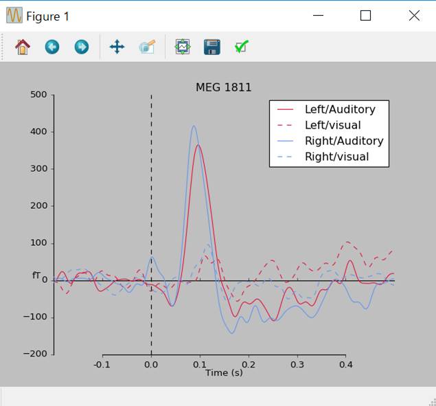
振幅を色表示
evoked_r_aud.plot_image(picks=picks)
全チャンネル表示です。縦軸はチャンネルです。振幅は色で表示されてます。ま、聴覚誘発は1エポックでも背景自発活動なみの振幅ありますから、こういう芸当ができます。背景自発活動と比べて小さい誘発活動の場合には使えません。
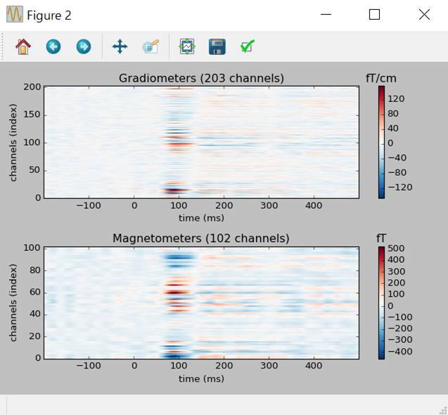
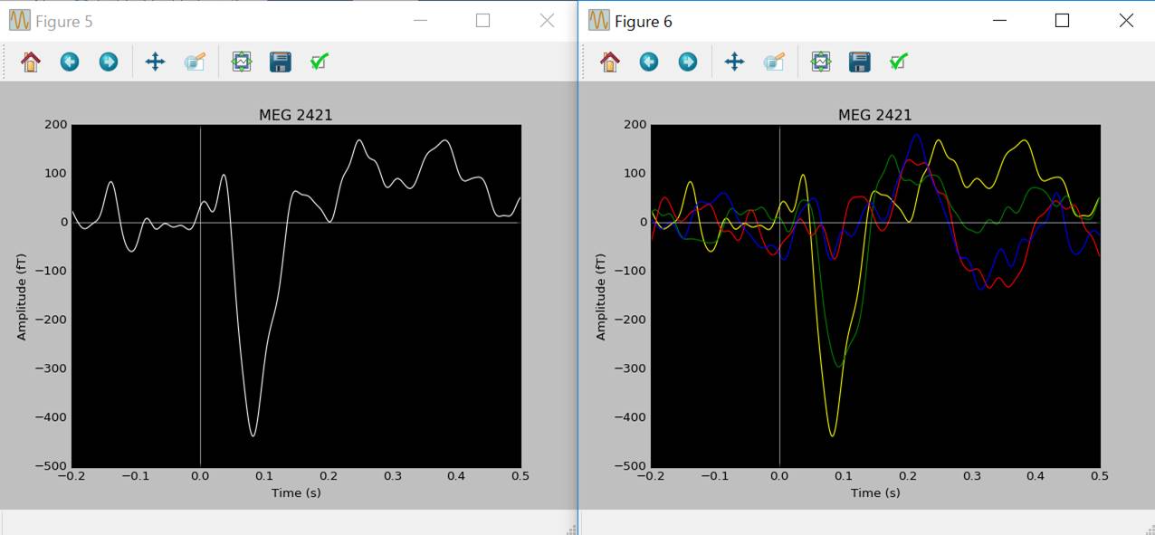
鳥瞰図表示
title='MNE
sample data (condition :%s)'
evoked_l_aud.plot_topo(title=title % evoked_l_aud.comment) #1個だけ表示
colors='yellow','green','red','blue'
mne.viz.plot_evoked_topo(evoked,color=colors,title=title % 'Left/Right Auditory/Visual') # 4個表示
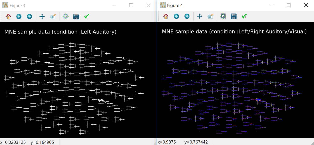
波形をクリックすればそのセンサの波形が拡大評価されます。
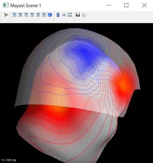
等磁場線図の三次元表示(実行不可)
subjects_dir=data_path+'\\subjects'
trans_fname=data_path+'\\MEG\\sample\\sample_audvis_raw-trans.fif'
# 座標変換行列
maps=mne.make_field_map(evoked_l_aud,trans=trans_fname,subject='sample',subjects_dir=subjects_dir,n_jobs=1)
field_map=evoked_l_aud.plot_field(maps,time=0.1)
エラーが出ます。
ImportError: No module named 'mayavi'
>>> Traceback (most recent call last):
File
"<stdin>", line 1, in <module>
mayaviのアナコンダ・パッケージはPython
2.7しか対応してないそうですんで諦めます。
Python
2.7.13とpython consoleで実行したとこ。
Jupyterやipythonだとうまく表示されません。