内容

L2ノルム推定... 1

準備... 1

脳磁図データ処理... 1

分散行列の規則化... 1

加算平均波形の計算... 1

逆問題を解く準備... 1

電流源推定... 1

結果表示（３Dは実行不可）... 1

単一電流双極子推定... 1

準備と各ファイル読み込み... 1

単一電流双極子推定... 1

結果表示（実行不可）... 1

計測データと計算データの比較... 1

電流双極子の経時変化... 1

MNE-Pythonのtutorialの以下の部分を試してみました。

L2ノルム推定

準備

import numpy as np

import matplotlib.pyplot as plt

import mne

from mne.datasets import sample

from mne.minimum_norm import (make_inverse_operator,apply_inverse,write_inverse_operator)

脳磁図データ処理

脳磁図の生データを読み込んでエポックの切り出しをします。

data_path=sample.data_path()

raw_fname=data_path+'\\MEG\\sample\\sample_audvis_filt-0-40_raw.fif'

raw=mne.io.read_raw_fif(raw_fname,add_eeg_ref=False)

raw.set_eeg_reference() # EEGの平均をreferenceとする

events=mne.find_events(raw,stim_channel='STI 014')

event_id=dict(aud_r=1) # event triggerと条件

tmin=-0.2

tmax=0.5

raw.info['bads']=['MEG 2443','EEG 053']

picks=mne.pick_types(raw.info,meg=True,eeg=False,eog=True,exclude='bads')

baseline=(None,0)

reject=dict(grad=4000e-13,mag=4e-12,eog=150e-6)

epochs=mne.Epochs(raw,events,event_id,tmin,tmax,proj=True,picks=picks,baseline=baseline,reject=reject,add_eeg_ref=False)

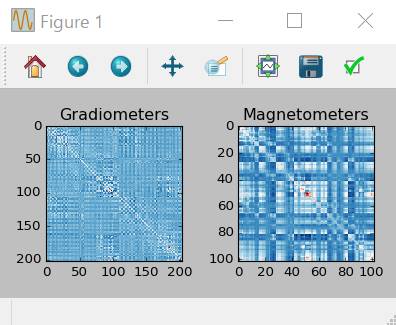
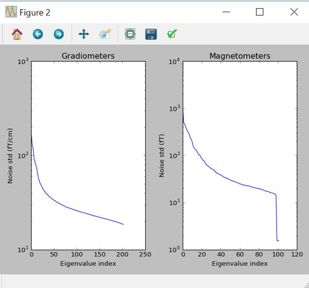
分散行列の規則化

noise_cov=mne.compute_covariance(epochs,tmax=0.,method=['shrunk','empirical'])

fig_cov,fig_spectra=mne.viz.plot_cov(noise_cov,raw.info)

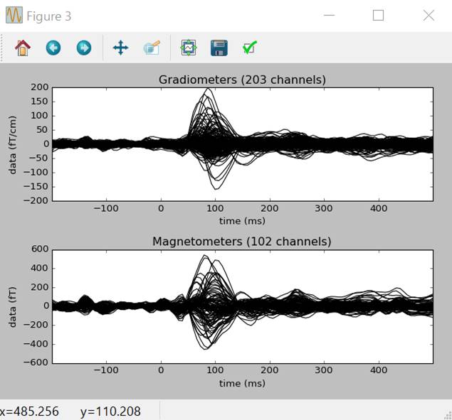
加算平均波形の計算

evoked=epochs.average()

evoked.plot()

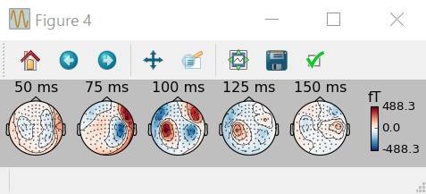
evoked.plot_topomap(times=np.linspace(0.05,0.15,5),ch_type='mag')

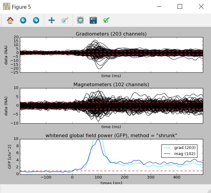
evoked.plot_white(noise_cov)

逆問題を解く準備

# 導体モデルの読み込み

fname_fwd=data_path+'\\MEG\\sample\\sample_audvis-meg-oct-6-fwd.fif'

fwd=mne.read_forward_solution(fname_fwd,surf_ori=True)

# 導体モデルを脳磁図だけにする

fwd=mne.pick_types_forward(fwd,meg=True,eeg=False)

# 逆問題を解く

info=evoked.info

inverse_operator=make_inverse_operator(info,fwd,noise_cov,loose=0.2,depth=0.8)

write_inverse_operator('sample_audvis-meg-oct-6-inv.fif',inverse_operator)

電流源推定

method='dSPM'

snr=3.

lambda2=1./snr**2

stc=apply_inverse(evoked,inverse_operator,lambda2,method=method,pick_ori=None)

# del fwd,inverse_operator,epochs # メモリ節約

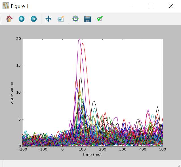
結果表示（３Dは実行不可）

plt.close('all') # ウインドウは全部閉じる

plt.plot(1e3*stc.times,stc.data[::100,:].T)

plt.xlabel('time (ms)')

plt.ylabel('%s value' % method)

plt.show()

三次元表示です。実行は・・・できませんでした。

vertno_max,time_max=stc.get_peak(hemi='rh')

subjects_dir=data_path+'\\subjects'

brain=stc.plot(surface='inflated',hemi='rh',subjects_dir=subjects_dir,clim=dict(kind='value',lims=[8,12,15]),initial_time=time_max,time_unit='s')

brain.add_foci(vertno_max,coords_as_verts=True,hemi='rh',color='blue',scale_factor=0.6)

brain.show_view('lateral')

File "C:\Users\akira\Anaconda3\lib\site-packages\mne\source_estimate.py", line 1334, in plot

time_unit=time_unit)

File "C:\Users\akira\Anaconda3\lib\site-packages\mne\viz\_3d.py", line 704, in plot_source_estimates

Traceback (most recent call last):

File "<stdin>", line 1, in <module>

import surfer

ImportError: No module named 'surfer'

module surferの導入を試みます。

Microsoft Windows [Version 10.0.14393]

(c) 2016 Microsoft Corporation. All rights reserved.

C:\Users\akira>pip install surfer

Collecting surfer

Could not find a version that satisfies the requirement surfer (from versions: )

No matching distribution found for surfer

C:\Users\akira>

導入できませんでした。

以下もmodule surferがないため実行できませんでした。

fs_vertices=[np.arange(10242)]*2

morph_mat=mne.compute_morph_matrix('sample','fsaverage',stc.vertices,fs_vertices,smooth=None,subjects_dir=subjects_dir)

stc_fsaverage=stc.morph_precomputed('fsaverage',fs_vertices,morph_mat)

brain_fsaverage=stc_fsaverage.plot(surface='inflated',hemi='rh',subjects_dir=subjects_dir,clim=dict(kind='value',lims=[8,12,15]),initial_time=time_max, time_unit='s')

brain_fsaverage.show_view('lateral')

単一電流双極子推定

準備と各ファイル読み込み

from os import path as op

import numpy as np

import matplotlib.pyplot as plt

plt.close('all')

import mne

from mne.forward import make_forward_dipole

from mne.evoked import combine_evoked

from mne.simulation import simulate_evoked

data_path=mne.datasets.sample.data_path()

subjects_dir=op.join(data_path,'subjects')

fname_ave=op.join(data_path,'MEG','sample','sample_audvis-ave.fif')

fname_cov=op.join(data_path,'MEG','sample','sample_audvis-cov.fif')

fname_bem=op.join(subjects_dir,'sample','bem','sample-5120-bem-sol.fif')

fname_trans=op.join(data_path,'MEG','sample','sample_audvis_raw-trans.fif')

fname_surf_lh=op.join(subjects_dir,'sample','surf','lh.white')

単一電流双極子推定

脳磁図データだけを使って単一電流双極子推定を行います。

evoked=mne.read_evokeds(fname_ave,condition='Right Auditory',baseline=(None,0))

evoked.pick_types(meg=True,eeg=False)

evoked_full=evoked.copy()

evoked.crop(0.07,0.08)

dip=mne.fit_dipole(evoked,fname_cov,fname_bem,fname_trans)[0]

結果表示（実行不可）

結果の表示ですが、できません。module mayaviのPython 3対応待ちです。

dip.plot_locations(fname_trans,'sample',subjects_dir)

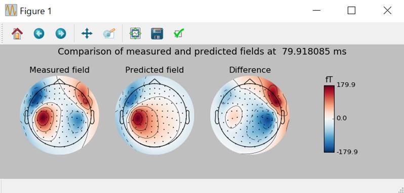
計測データと計算データの比較

GOF最高時点の等磁場線図の比較をします。

fwd,stc=make_forward_dipole(dip,fname_bem,evoked.info,fname_trans)

pred_evoked=simulate_evoked(fwd,stc,evoked.info,None,snr=np.inf)

# GOF最高点の時間

best_idx=np.argmax(dip.gof)

best_time=dip.times[best_idx]

# 図の表示準備

fig,axes=plt.subplots(nrows=1,ncols=4,figsize=[10.,3.4])

vmin,vmax=-400,400 # 色表示のスケール

# GOF最高時間のトポグラフィ表示

plot_params=dict(times=best_time,ch_type='mag',outlines='skirt',colorbar=False)

evoked.plot_topomap(time_format='Measured field',axes=axes[0],**plot_params)

# 計算画像との比較

pred_evoked.plot_topomap(time_format='Predicted field',axes=axes[1],**plot_params)

# 差分

diff=combine_evoked([evoked,-pred_evoked],weights='equal')

plot_params['colorbar']=True

diff.plot_topomap(time_format='Difference',axes=axes[2],**plot_params)

plt.suptitle('Comparison of measured and predicted fields at {: 0f} ms'.format(best_time*1000.),fontsize=16)

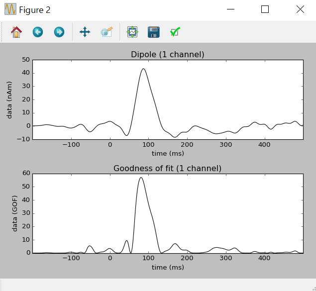
電流双極子の経時変化

dip_fixed=mne.fit_dipole(evoked_full,fname_cov,fname_bem,fname_trans,pos=dip.pos[best_idx],ori=dip.ori[best_idx])[0]

dip_fixed.plot()