In [1]:
import sys
print(sys.version_info)
del sys
dSPM
準備
In [2]:
import numpy as np
import matplotlib.pyplot as plt
import mne
from mne.datasets import sample
from mne.minimum_norm import (make_inverse_operator,apply_inverse,write_inverse_operator)
mne.set_log_level('INFO')
data_path=sample.data_path()
raw_fname=data_path+'\\MEG\\sample\\sample_audvis_filt-0-40_raw.fif'
In [3]:
raw=mne.io.read_raw_fif(raw_fname)
raw.set_eeg_reference()
events=mne.find_events(raw,stim_channel='STI 014')

event_id=dict(aud_r=1)
tmin=-0.2
tmax=0.5
raw.info['bads']=['MEG 2443','EEG 053']
picks=mne.pick_types(raw.info,meg=True,eeg=False,eog=True,exclude='bads')
baseline=(None,0)
reject=dict(grad=4000e-13,mag=4e-12,eog=150e-6)
epochs=mne.Epochs(raw,events,event_id,tmin,tmax,proj=True,picks=picks,baseline=baseline,reject=reject)
分散行列の計算
In [4]:
noise_cov=mne.compute_covariance(epochs,tmax=0.,method=['shrunk','empirical'])
print(noise_cov.data.shape)
fig_cov,fig_spectra=mne.viz.plot_cov(noise_cov,raw.info);


加算波形の表示
In [5]:
evoked=epochs.average()
evoked.plot()
evoked.plot_topomap(times=np.linspace(0.05,0.15,5),ch_type='mag');
evoked.plot_white(noise_cov);


逆問題を解く準備
導体モデルは予めFreeSurferで計算したメッシュを使います。
In [6]:
# 導体モデル読み込み
fname_fwd=data_path+'\\MEG\\sample\\sample_audvis-meg-oct-6-fwd.fif'

# 順問題を解く
fwd=mne.read_forward_solution(fname_fwd,surf_ori=True)
print(fwd)
fwd=mne.pick_types_forward(fwd,meg=True,eeg=False)
print(fwd)
print(fwd.keys())

# 逆問題を解く
info=evoked.info
inverse_operator=make_inverse_operator(info,fwd,noise_cov,loose=0.2,depth=0.8)
print(inverse_operator.keys())
write_inverse_operator('sample_audvis-meg-oct-6-inv.fif',inverse_operator)
In [7]:
# inverse_operator
print(inverse_operator['eigen_fields'])
print(inverse_operator['eigen_leads_weighted'])
print(inverse_operator['fmri_prior'])
print(inverse_operator['orient_prior'])
print(inverse_operator['mri_head_t'])
print(inverse_operator['sing'].shape)
print(inverse_operator['nsource'])
print(inverse_operator['info'])
print(inverse_operator['src'])
print(inverse_operator['source_cov'])
print(inverse_operator['eigen_leads'])
逆問題を解く
In [8]:
method='dSPM'
snr=3.
lambda2=1./snr**2
stc=apply_inverse(evoked,inverse_operator,lambda2,method=method,pick_ori=None)
# del fwd,inverse_operator,epochs # メモリ節約
In [9]:
plt.plot(1e3*stc.times,stc.data[::100,:].T)
plt.xlabel('time (ms)')
plt.ylabel('%s value' % method)
plt.show()

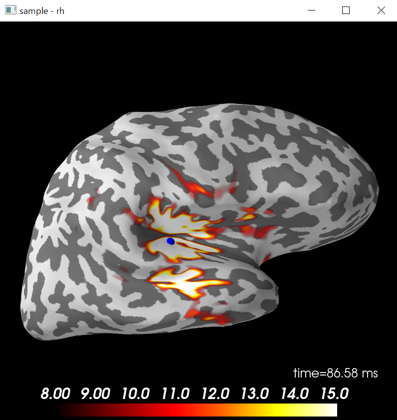
In [10]:
# jupyterでは実行できず
vertno_max,time_max=stc.get_peak(hemi='rh')
subjects_dir=data_path+'\\subjects'
clim=dict(kind='value',lims=[8,12,15])
# inflated brainが出現
brain=stc.plot(surface='inflated',hemi='rh',subjects_dir=subjects_dir,clim=clim,initial_time=time_max,time_unit='s')
# 青い点が出現
brain.add_foci(vertno_max,coords_as_verts=True,hemi='rh',color='blue',scale_factor=0.6)
brain.show_view('lateral')
Out[10]:
python consoleでは以下のような絵ができます。

青点表示時
In [11]:
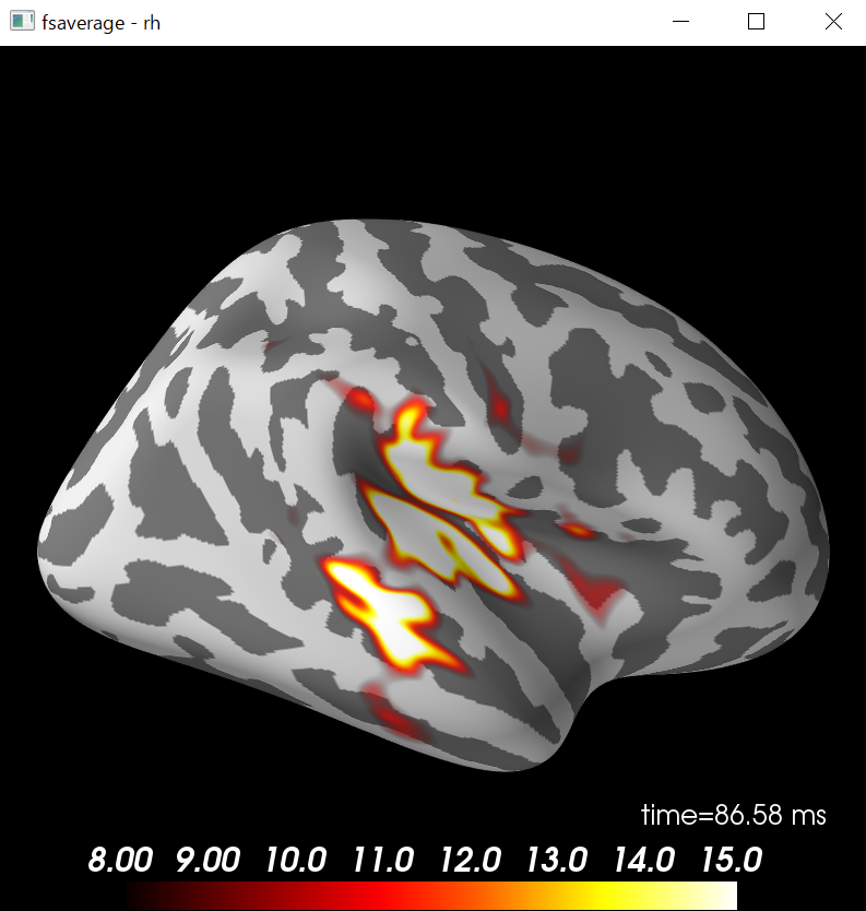
fs_vertices=[np.arange(10242)]*2
morph_mat=mne.compute_morph_matrix('sample','fsaverage',stc.vertices,fs_vertices,smooth=None,subjects_dir=subjects_dir)
print(morph_mat.shape)
stc_fsaverage=stc.morph_precomputed('fsaverage',fs_vertices,morph_mat)
brain_fsaverage=stc_fsaverage.plot(surface='inflated',hemi='rh',subjects_dir=subjects_dir,clim=clim,initial_time=time_max,time_unit='s')
brain_fsaverage.show_view('lateral')
Out[11]:
7498頂点を20484頂点に変換しています。
単一等価電流双極子推定
In [12]:
% reset
準備
In [13]:
import numpy as np
import matplotlib.pyplot as plt
import mne
mne.set_log_level('INFO')
from mne.forward import make_forward_dipole
from mne.evoked import combine_evoked
from mne.simulation import simulate_evoked

data_path=mne.datasets.sample.data_path()
subjects_dir=data_path+'\\subjects'
fname_ave=data_path+'\\MEG\\sample\\sample_audvis-ave.fif'
fname_cov=data_path+'\\MEG\\sample\\sample_audvis-cov.fif'
fname_bem=subjects_dir+'\\sample\\bem\\sample-5120-bem-sol.fif'
fname_trans=data_path+'\\MEG\\sample\\sample_audvis_raw-trans.fif'
fname_surf_lh=subjects_dir+'\\sample\\surf\\lh.white'
単一等価電流双極子推定
In [14]:
evoked=mne.read_evokeds(fname_ave,condition='Right Auditory',baseline=(None,0))
evoked.pick_types(meg=True,eeg=False)
evoked_full=evoked.copy() # pythonは参照なので・・・
evoked.crop(0.07,0.08)

dip=mne.fit_dipole(evoked,fname_cov,fname_bem,fname_trans)
In [15]:
print(dip[0])
print(dip[1].shape)
print(len(dip[0]))
print(dip[0][0].times)
print(dip[0][0].pos)
print(dip[0][0].amplitude)
print(dip[0][0].ori)
print(dip[0][0].gof)
print(dip[0][0].name)
print(dip[1].shape)
In [16]:
# jupyterでも描画
dip[0].plot_locations(fname_trans,'sample',subjects_dir,mode='orthoview');

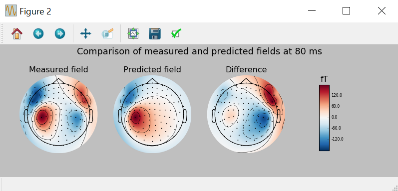
計測磁場と計算磁場
In [17]:
fwd,stc=make_forward_dipole(dip[0],fname_bem,evoked.info,fname_trans)
pred_evoked=simulate_evoked(fwd,stc,evoked.info,None,snr=np.inf)
In [18]:
# jupyterだとうまく表示できず
%matplotlib inline
# 高いGOF時点の検出
best_idx=np.argmax(dip[0].gof)
best_time=dip[0].times[best_idx]

# subplot用のcolorbar
fig,axes=plt.subplots(nrows=1,ncols=4,figsize=[10.,3.5]); # どうも調子悪いです。
vmin,vmax=-400,400

plot_params=dict(times=best_time,ch_type='mag',outlines='skirt',colorbar=False);
evoked.plot_topomap(time_format='Measured field',axes=axes[0],**plot_params);
pred_evoked.plot_topomap(time_format='Predicted field',axes=axes[1],**plot_params);

diff=combine_evoked([evoked,-pred_evoked],weights='equal');
plot_params['colorbar'] = True
diff.plot_topomap(time_format='Difference',axes=axes[2],**plot_params);

plt.suptitle('Comparison of measured and predicted fields at {:.0f} ms'.format(best_time*1000.),fontsize=16);


どうも調子悪いです。
python consoleだと以下のようになります。
In [19]:
dip_fixed=mne.fit_dipole(evoked_full,fname_cov,fname_bem,fname_trans,pos=dip[0].pos[best_idx],ori=dip[0].ori[best_idx])[0]
dip_fixed.plot();
