BrainVISAの結果をMNE-Cで使う方法２

NiBabelのインストール... 1

Spyder (mne)の起動... 1

NIfTIの書き換え... 1

GIfTIの書き換え... 1

「BrainVISAの結果をMNE-Cで使う方法」http://meg.aalip.jp/python/BrainVISA_MNE.htm

はMATLABを使いましたが、そのPython版です。

変更点のみ記しています。

NiBabelのインストール

PythonでNIfTIやGIfTIの読み書きを行うにはNiBabelを使います。

本来Python 3.xでは三次元表示をおこなうPython2.7用のMayaviを使用するのは難しいのですが、MNE-python 0.16以降をインストールすることで解決しています。MNE-python 0.16がインストールされている状態のPython 3.6以降での話とします。Python 2.7を使う場合にはMNE-python 0.16のインストールは不要です。

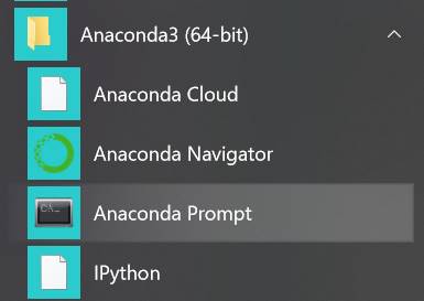
Anaconda Promptを起動します。

Anacondaとpythonのversionです。

(base) C:\Users\akira>conda --version && python --version

conda 4.5.11

Python 3.6.5 :: Anaconda, Inc.

NiBabelをインストールします。途中でyを押します。

(base) C:\Users\akira>conda install -c conda-forge nibabel

Solving environment: done

## Package Plan ##

environment location: C:\Users\akira\Anaconda3.6

added / updated specs:

- nibabel

The following packages will be downloaded:

package | build

---------------------------|-----------------

pydicom-1.1.0 | py_0 5.2 MB conda-forge

certifi-2018.4.16 | py36_0 143 KB conda-forge

nibabel-2.3.0 | pyh24bf2e0_1 2.7 MB conda-forge

conda-4.5.11 | py36_0 654 KB conda-forge

------------------------------------------------------------

Total: 8.7 MB

The following NEW packages will be INSTALLED:

nibabel: 2.3.0-pyh24bf2e0_1 conda-forge

pydicom: 1.1.0-py_0 conda-forge

The following packages will be UPDATED:

certifi: 2018.4.16-py36_0 --> 2018.4.16-py36_0 conda-forge

conda: 4.5.11-py36_0 --> 4.5.11-py36_0 conda-forge

Proceed ([y]/n)? y

Downloading and Extracting Packages

pydicom-1.1.0 | 5.2 MB | ############################################################################ | 100%

certifi-2018.4.16 | 143 KB | ############################################################################ | 100%

nibabel-2.3.0 | 2.7 MB | ############################################################################ | 100%

conda-4.5.11 | 654 KB | ############################################################################ | 100%

Preparing transaction: done

Verifying transaction: done

Executing transaction: done

(base) C:\Users\akira>

動作確認をします。

(base) C:\Users\akira>python

Python 3.6.5 |Anaconda, Inc.| (default, Mar 29 2018, 13:32:41) [MSC v.1900 64 bit (AMD64)] on win32

Type "help", "copyright", "credits" or "license" for more information.

>>> import nibabel

C:\Users\akira\Anaconda3.6\lib\site-packages\h5py\__init__.py:36: FutureWarning: Conversion of the second argument of issubdtype from `float` to `np.floating` is deprecated. In future, it will be treated as `np.float64 == np.dtype(float).type`.

from ._conv import register_converters as _register_converters

>>>

認識されました。

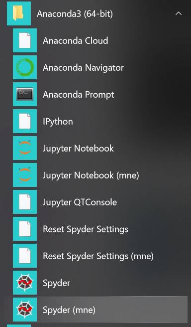
Spyder (mne)の起動

mneをactivateしたSpyder (mne)を起動します。

以下を実行します。

fimport numpy as np

import matplotlib.pyplot as plt #描画用

import nibabel as nib

結果です。

Python 3.6.6 |Anaconda, Inc.| (default, Jun 28 2018, 11:27:44) [MSC v.1900 64 bit (AMD64)]

Type "copyright", "credits" or "license" for more information.

IPython 6.5.0 -- An enhanced Interactive Python.

In [1]: from mayavi import mlab

...: import numpy as np

...: import matplotlib.pyplot as plt #描画用

...: import nibabel as nib

MayaviのバックエンドをQt4に変更しています

In [2]:

NIfTIの書き換え

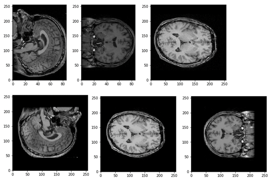
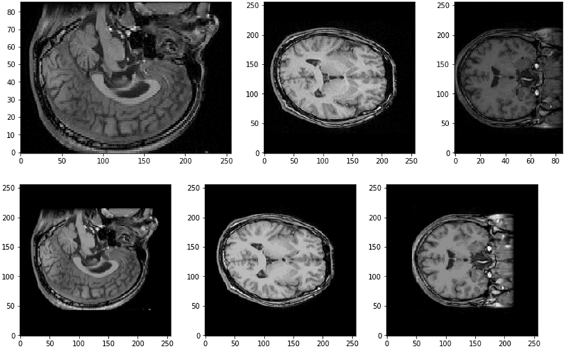
BrainVISAとFreeSurferの座標の違いを示します。以下を実行します。

a_T1=nib.load('c:\\test\\a\\mri\\T1.nii.gz')

a_brain=nib.load('c:\\test\\a\\mri\\brain.nii.gz')

b_T1=nib.load('c:\\test\\b\\mri\\T1.nii.gz')

for T1 in [a_T1,b_T1]:

scale=np.linalg.norm(T1.affine[0:3,0:3],axis=1)

img0=T1.get_data()

sz=round(img0.shape[0]/2)

aspect=scale[1]/scale[2]

plt.imshow(img0[sz,:,:],aspect=aspect,cmap='gray',origin='lower')

plt.show()

sz=round(img0.shape[1]/2);

aspect=scale[0]/scale[2]

plt.imshow(img0[:,sz,:],aspect=aspect,cmap='gray',origin='lower')

plt.show()

sz=round(img0.shape[2]/2);

aspect=scale[0]/scale[1]

plt.imshow(img0[:,:,sz],aspect=aspect,cmap='gray',origin='lower')

plt.show()

マスクa_brainと頭部a_T1を掛け合わせ、脳実質を抽出データに変換します。

img0=a_T1.get_data()

img1=a_brain.get_data()

img1[img1>0]=1

img1[img1<1]=0

img1=img1*img0

NIfTIデータの書き換えを行います。MATLABのniftiwrite関数と違ってnib.save(データ、アッフィン変換)だけでOKです。

sz=img0.shape

new_data=np.arange(img0.size,dtype=np.int16)

new_data=new_data.reshape([sz[0],sz[2],sz[1]])

data=img0

for z in range(sz[2]):

new_data[:,z,:]=data[:,:,sz[2]-z-1]

affine=a_T1.affine.copy().T

pixscale=np.linalg.norm(affine,axis=1)

affine[:,1]=a_T1.affine[2,:]

affine[:,2]=a_T1.affine[1,:]

affine[2,1]=-affine[2,1]

affine[3,1]=-affine[3,1]+affine[2,1]

affine[:,0:2]=-affine[:,0:2]

affine[0,0]=-affine[0,0]

affine[3,0]=data.shape[0]*scale[0]/2;

affine=affine.T

array_img=nib.Nifti1Image(new_data,affine)

nib.save(array_img,'c:\\test\\a\\mri\\newT1.nii.gz')

data=img1

for z in range(sz[2]):

new_data[:,z,:]=data[:,:,sz[2]-z-1]

array_img=nib.Nifti1Image(new_data,affine)

nib.save(array_img,'c:\\test\\a\\mri\\newbrain.nii.gz')

確認してみます。

for T1 in [a_newT1,b_T1]:

scale=np.linalg.norm(T1.affine[0:3,0:3],axis=1)

img0=T1.get_data()

sz=round(img0.shape[0]/2)

aspect=scale[1]/scale[2]

plt.imshow(img0[sz,:,:],aspect=aspect,cmap='gray',origin='lower')

plt.show()

sz=round(img0.shape[1]/2);

aspect=scale[0]/scale[2]

plt.imshow(img0[:,sz,:],aspect=aspect,cmap='gray',origin='lower')

plt.show()

sz=round(img0.shape[2]/2);

aspect=scale[0]/scale[1]

plt.imshow(img0[:,:,sz],aspect=aspect,cmap='gray',origin='lower')

plt.show()

座標が揃いました。

GIfTIの書き換え

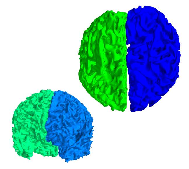
BrainVISAとFreeSurferの座標の違いを示します。

from mayavi import mlab

import numpy as np

import nibabel as nib

a_T1=nib.load('c:\\test\\a\\mri\\T1.nii.gz')

a_Lwhite=nib.load('C:\\test\\a\\surf\\Lwhite.gii')

a_Rwhite=nib.load('C:\\test\\a\\surf\\Rwhite.gii')

b_Lwhite=nib.load('C:\\test\\b\\surf\\lh.white.gii')

b_Rwhite=nib.load('C:\\test\\b\\surf\\rh.white.gii')

mlab.figure(bgcolor=(1,1,1))

# BrainVISA x座標は反転

p=a_Lwhite.darrays[0].data

mesh=a_Lwhite.darrays[1].data

mlab.triangular_mesh(-p[:,0],p[:,1],p[:,2],mesh,color=(0,0,1))

p=a_Rwhite.darrays[0].data

mesh=a_Rwhite.darrays[1].data

mlab.triangular_mesh(-p[:,0],p[:,1],p[:,2],mesh,color=(0,1,0))

# FreeSurfer x座標は反転せず

p=b_Lwhite.darrays[0].data

mesh=b_Lwhite.darrays[1].data

mlab.triangular_mesh(p[:,0],p[:,1],p[:,2],mesh,color=(0,0.5,1))

p=b_Rwhite.darrays[0].data

mesh=b_Rwhite.darrays[1].data

mlab.triangular_mesh(p[:,0],p[:,1],p[:,2],mesh,color=(0,1,0.5))

mlab.show()

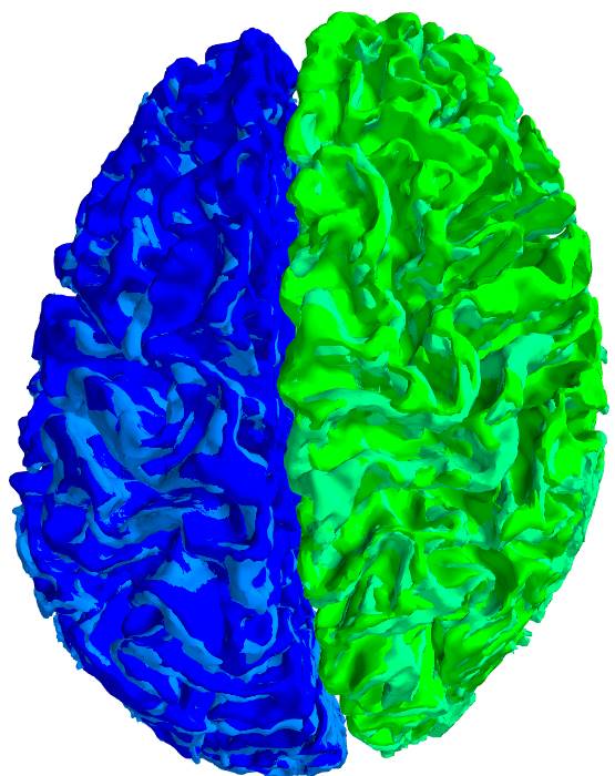
上がBrainVISA、下がFreeSurferです。

座標変換を行います。

dsize=np.array(np.mat(a_T1.shape))

pixscale=np.linalg.norm(a_T1.affine[0:3,0:3],axis=1)

d=dsize*pixscale

# X0=np.array([[1,0,0,-d[0,0]/2],[0,1,0,-d[0,1]/2],[0,0,1,-d[0,2]/2],[0,0,0,1]])

X0=np.array([[1,0,0,0],[0,1,0,0],[0,0,1,0],[-d[0,0]/2,-d[0,1]/2,-d[0,2]/2,1]])

X1=np.array([[-1.,0,0,0],[0,-1,0,0],[0,0,-1,0],[0,0,0,1]])

X2=np.dot(X0,X1)

for surf in [a_Lwhite,a_Rwhite]:

p=np.ones((surf.darrays[0].data.shape[0],4))

p[:,0:3]=surf.darrays[0].data.copy()

p=np.dot(p,X2)

surf.darrays[0].data[:,:]=p[:,0:3]# data=p[:,0:3]は不可

f=surf.darrays[1].data.copy()

surf.darrays[1].data[:,1]=f[:,2]

surf.darrays[1].data[:,2]=f[:,1]

nib.save(a_Lwhite,'C:\\test\\a\\surf\\newLwhite.gii')

nib.save(a_Rwhite,'C:\\test\\a\\surf\\newRwhite.gii')

確認します。

a_newLwhite=nib.load('C:\\test\\a\\surf\\newLwhite.gii')

a_newRwhite=nib.load('C:\\test\\a\\surf\\newRwhite.gii')

mlab.figure(bgcolor=(1,1,1))

# BrainVISAを座標変換 x座標は反転させず

p=a_newLwhite.darrays[0].data

mesh=a_newLwhite.darrays[1].data

mlab.triangular_mesh(p[:,0],p[:,1],p[:,2],mesh,color=(0,0,1))

p=a_newRwhite.darrays[0].data

mesh=a_newRwhite.darrays[1].data

mlab.triangular_mesh(p[:,0],p[:,1],p[:,2],mesh,color=(0,1,0))

# FreeSurfer x座標は反転せず

p=b_Lwhite.darrays[0].data

mesh=b_Lwhite.darrays[1].data

mlab.triangular_mesh(p[:,0],p[:,1],p[:,2],mesh,color=(0,0.5,1))

p=b_Rwhite.darrays[0].data

mesh=b_Rwhite.darrays[1].data

mlab.triangular_mesh(p[:,0],p[:,1],p[:,2],mesh,color=(0,1,0.5))

mlab.show()

座標が一致し、BrainVISAとFreeSurferのポリゴンメッシュがほぼ重なりました。ポリゴンメッシュそのものは異なっているので脳回の模様に微妙にムラがあります。