Contents
球面上の三角形の面積
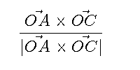
理屈は考えず、公式集の結果だけを使います。 http://hooktail.sub.jp/vectoranalysis/SphereTriangle/ などを参考にしました。 原点をOとし、半径1の球面上の点A、B、Cがあり、∠AOBをc、∠AOCをb、∠BOCをaとします。 球面上の∠BAC(内角)をαとし、平面AOBと平面AOCの為す角とします。 平面AOBの平面AOCの為す角は平面AOBと平面AOCの法線の為す角とします。 平面AOCの単位法線はOAとOCの外積の規格化したものとします。
figure('color',[1,1,1],'position',[50,50,200,100]);
st='$$\frac{\vec{OA}\times\vec{OC}}{|\vec{OA}\times\vec{OC}|}$$';
text(0,0.5,st,'interpreter','latex','Fontsize',18);
axis off;
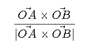
平面AOBの単位法線はOAとOBの外積を規格化したものとします。
figure('color',[1,1,1],'position',[50,50,200,100]);
st='$$\frac{\vec{OA}\times\vec{OB}}{|\vec{OA}\times\vec{OB}|}$$';
text(0,0.5,st,'interpreter','latex','Fontsize',18);
axis off;
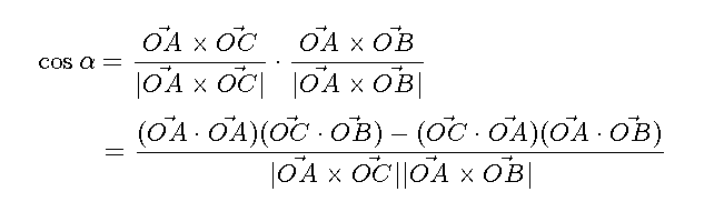
内角BACは平面AOCと平面AOBの法線の為す角ということで内積を用います。 外積と内積の公式を使ってカッコを展開します。
close all;
figure('color',[1,1,1],'position',[50,50,650,200]);
st1='$$\cos\alpha=\frac{\vec{OA}\times\vec{OC}}{|\vec{OA}\times\vec{OC}|}\cdot\frac{\vec{OA}\times\vec{OB}}{|\vec{OA}\times\vec{OB}|}$$';
st2='$$=\frac{(\vec{OA}\cdot\vec{OA})(\vec{OC}\cdot\vec{OB})-(\vec{OC}\cdot\vec{OA})(\vec{OA}\cdot\vec{OB})}{|\vec{OA}\times\vec{OC}||\vec{OA}\times\vec{OB}|}$$';
text(-0.1,0.75,st1,'interpreter','latex','Fontsize',18);
text(0.02,0.25,st2,'interpreter','latex','Fontsize',18);
axis off;
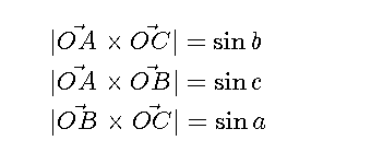
半径は1なので外積はsinだけとなり、絶対値のところは以下のようにかけます。
figure('color',[1,1,1],'position',[50,50,350,150]);
st1='$$|\vec{OA}\times\vec{OC}|=\sin b$$';
st2='$$|\vec{OA}\times\vec{OB}|=\sin c$$';
st3='$$|\vec{OB}\times\vec{OC}|=\sin a$$';
text(0,0.8,st1,'interpreter','latex','Fontsize',18);
text(0,0.5,st2,'interpreter','latex','Fontsize',18);
text(0,0.2,st3,'interpreter','latex','Fontsize',18);
axis off;
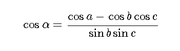
内積・外積をcos、sinで書き換えます。
figure('color',[1,1,1],'position',[50,50,350,100]);
st='$$\cos\alpha=\frac{\cos a -\cos b \cos c}{\sin b \sin c}$$';
text(0,0.5,st,'interpreter','latex','Fontsize',18);
axis off;
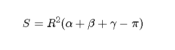
球面上の三角形の面積Sは、内角をα、β、γ、半径をRとすると以下の公式が使えます。
figure('color',[1,1,1],'position',[50,50,350,100]);
st='$$S=R^2(\alpha+\beta+\gamma-\pi)$$';
text(0,0.5,st,'interpreter','latex','Fontsize',18);
axis off;
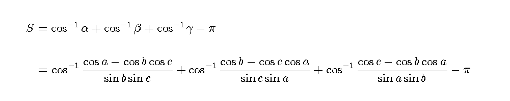
半径1のときの球面上の3点ABCが為す三角形の面積は以下の通りになります。
close all;
figure('color',[1,1,1],'position',[50,50,1000,200]);
st1='$$S=\cos^{-1}\alpha+\cos^{-1}\beta+\cos^{-1}\gamma-\pi$$';
st2='$$=\cos^{-1}\frac{\cos a - \cos b \cos c}{\sin b \sin c}+\cos^{-1}\frac{\cos b - \cos c \cos a}{\sin c \sin a}+\cos^{-1}\frac{\cos c - \cos b \cos a}{\sin a \sin b}-\pi$$';
text(-0.1,0.75,st1,'interpreter','latex','Fontsize',18);
text(-0.07,0.25,st2,'interpreter','latex','Fontsize',18);
axis off;
メッシュの内外判定
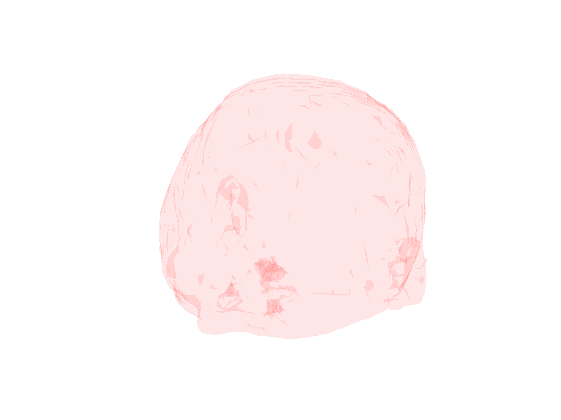
ある点が三角メッシュの内か外かの判定は、その点を中心とした各三角メッシュの立体角の総和が±4π,±12π,±20π・・・かどうかとなります。 MATLABにあるmriファイルで試してみます。 isosurface関数を使ってメッシュを作成しますが、そのままだとメッシュが閉じてくれないので、蓋を作るべく、上下にゼロ行列を挿入します。
clear;close all;
load mri;
D=squeeze(D);
D0=repmat(uint8(0),[siz(1),siz(2),1]);
D=cat(3,D0,D,D0);
hmesh=isosurface(D,1);
hmesh=reducepatch(hmesh,5000);
hmesh.vertices(:,3)=hmesh.vertices(:,3)*2.5;
figure('color',[1,1,1]);
hskull=patch(hmesh,'edgecolor','none','facecolor',[1,0.5,0.5]);
set(hskull,'facealpha',0.1);hold on;
daspect([1,1,1]);
axis off;axis tight;
rotate3d on;view([40,25]);
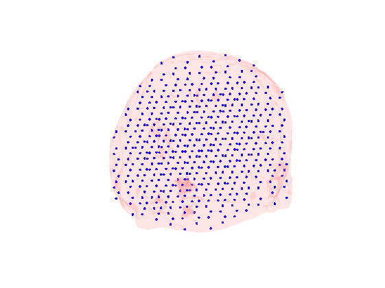
1cmおきに格子点を設け、メッシュの内外判定を行い、メッシュの内側だけ表示させます。
sg=10;
limx=round(xlim/sg)*sg;
limy=round(ylim/sg)*sg;
limz=round(zlim/sg)*sg;
limx=min(limx):sg:max(limx);
limy=min(limy):sg:max(limy);
limz=min(limz):sg:max(limz);
[x,y,z]=meshgrid(limx,limy,limz);
P=[x(:),y(:),z(:)];
S=zeros(size(P,1),1);
N=size(P,1);
pt=1:N;
nv=size(hmesh.vertices,1);
for n=1:N
    p=hmesh.vertices-ones(nv,1)*P(n,:);
    p=p./(sum(p.^2,2).^0.5*ones(1,3));
    p1=p(hmesh.faces(:,1),:);
    p2=p(hmesh.faces(:,2),:);
    p3=p(hmesh.faces(:,3),:);
    ang1=acos(sum(p1.*p2,2));
    ang2=acos(sum(p2.*p3,2));
    ang3=acos(sum(p3.*p1,2));
    ca1=cos(ang1);sa1=sin(ang1);
    ca2=cos(ang2);sa2=sin(ang2);
    ca3=cos(ang3);sa3=sin(ang3);
    s=acos((ca1-ca2.*ca3)./(sa2.*sa3))+acos((ca2-ca3.*ca1)./(sa3.*sa1))+acos((ca3-ca2.*ca1)./(sa1.*sa2))-pi;
    s=sum(s)/pi;
    S(n)=s;
    if s<3.95
        pt(n)=0;
    end;
end;
pt(pt==0)=[];
plot3(P(pt,1),P(pt,2),P(pt,3),'b.');
daspect([1,1,1]);view([40,25]);
rotate3d on;
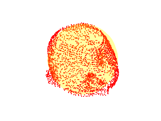
頭皮メッシュから仮想球を作成
頭皮メッシュから仮想球を作成します。
figure('color',[1,1,1],'position',[50,50,500,50]);
st='$$x^2+y^2+z^2+ax+by+cz+d=0$$';
text(-0.1,0.5,st,'interpreter','latex','fontsize',18);axis off;

%という球を仮定します。変形します。
figure('color',[1,1,1],'position',[50,50,500,50]);
st='$$ax+by+cz+d=-(x^2+y^2+z^2)$$';
text(-0.1,0.5,st,'interpreter','latex','fontsize',18);axis off;

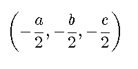
%x,y,zは頭皮の座標になります。a,b,c,dは行列の割り算で簡単に求まります。
% 球の中心は
figure('color',[1,1,1],'position',[50,50,200,100]);
st='$$\left(-\frac{a}{2},-\frac{b}{2},-\frac{c}{2}\right)$$';
text(-0.1,0.5,st,'interpreter','latex','fontsize',18);axis off;
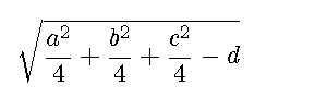
となります。また半径は
figure('color',[1,1,1],'position',[50,50,300,100]);
st='$$\sqrt{\frac{a^2}{4}+\frac{b^2}{4}+\frac{c^2}{4}-d}$$';
text(-0.1,0.5,st,'interpreter','latex','fontsize',18);axis off;
となります。 実際に試してみます。
figure('color',[1,1,1]);
p=hmesh.vertices;
plot3(p(:,1),p(:,2),p(:,3),'r.');hold on;
axis equal;axis tight;axis off;
q=[p,ones(size(p,1),1)]\(-sum(p.^2,2));
c0=-q(1:3)/2;
r=sqrt(sum(c0.^2)-q(4));
[sx,sy,sz]=sphere(20);
sx=sx*r+c0(1);
sy=sy*r+c0(2);
sz=sz*r+c0(3);
h0=surf(sx,sy,sz,'facecolor',[1,1,0],'facealpha',0.2,'edgecolor','none');
rotate3d on;