Contents
球面調和関数の式
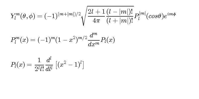
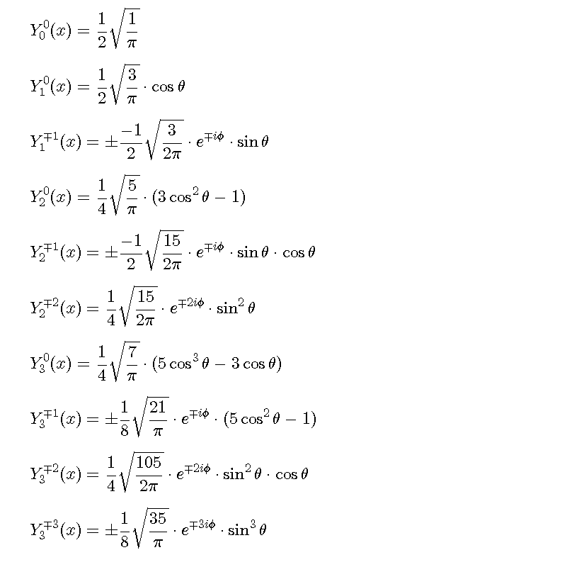
球面調和関数は球座標版のフーリエ変換です。 式の中にルジャンドル(Legendre)陪関数を含みます。 ルジャンドル陪関数はルジャンドル多項式を含みます。 式は以下の通り複雑です。
close all;clear all;
fs='FontSize';
figure('color',[1,1,1],'position',[50,50,800,400]);
st1='$$Y ^m _l (\theta, \phi)=(-1)^{(m+|m|)/2} \sqrt{\frac{2l+1}{4\pi}\frac{(l-|m|)!}{(l+|m|)!}}';
st2=' P^{|m|}_l (cos\theta) e^{im\phi}$$';
st3='$$P^{m}_{l}(x)=(-1)^m(1-x^2)^{m/2}\frac{d^m}{dx^m}P_l(x)$$';
st4='$$P_{l}(x)=\frac{1}{2^ll!}\frac{d^l}{dl^l}\left[(x^2-1)^l\right]$$';
text(-0.1,0.9,[st1,st2],'interpreter','latex',fs,20);
text(-0.1,0.6,st3,'interpreter','latex',fs,20);
text(-0.1,0.3,st4,'interpreter','latex',fs,20);
axis tight;axis off;
figure('color',[1,1,1],'position',[50,50,800,800]');
st{1}='$$Y^0_0(x)=\frac{1}{2}\sqrt{\frac{1}{\pi}}$$';
st{2}='$$Y^0_1(x)=\frac{1}{2}\sqrt{\frac{3}{\pi}}\cdot\cos\theta$$';
st{3}='$$Y^{\mp1}_1(x)=\pm\frac{-1}{2}\sqrt{\frac{3}{2\pi}}\cdot e^{\mp i\phi}\cdot\sin\theta$$';
st{4}='$$Y^0_2(x)=\frac{1}{4}\sqrt{\frac{5}{\pi}}\cdot(3\cos^2\theta-1)$$';
st{5}='$$Y^{\mp1}_2(x)=\pm\frac{-1}{2}\sqrt{\frac{15}{2\pi}}\cdot e^{\mp i\phi}\cdot\sin\theta\cdot\cos\theta$$';
st{6}='$$Y^{\mp2}_2(x)=\frac{1}{4}\sqrt{\frac{15}{2\pi}}\cdot e^{\mp2i\phi}\cdot\sin^2\theta$$';
st{7}='$$Y^0_3(x)=\frac{1}{4}\sqrt{\frac{7}{\pi}}\cdot (5\cos^3\theta-3\cos\theta)$$';
st{8}='$$Y^{\mp1}_3(x)=\pm\frac{1}{8}\sqrt{\frac{21}{\pi}}\cdot e^{\mp i\phi}\cdot (5\cos^2\theta-1)$$';
st{9}='$$Y^{\mp2}_3(x)=\frac{1}{4}\sqrt{\frac{105}{2\pi}}\cdot e^{\mp2i\phi}\cdot\sin^2\theta\cdot\cos\theta$$';
st{10}='$$Y^{\mp3}_3(x)=\pm\frac{1}{8}\sqrt{\frac{35}{\pi}}\cdot e^{\mp3i\phi}\cdot\sin^3\theta$$';
for n=1:length(st)
    text(-0.1,1.15-0.12*n,st{n},'interpreter','latex','FontSize',18);
end;

axis off;
ルジャンドル陪関数(随伴関数)legendre
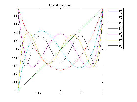
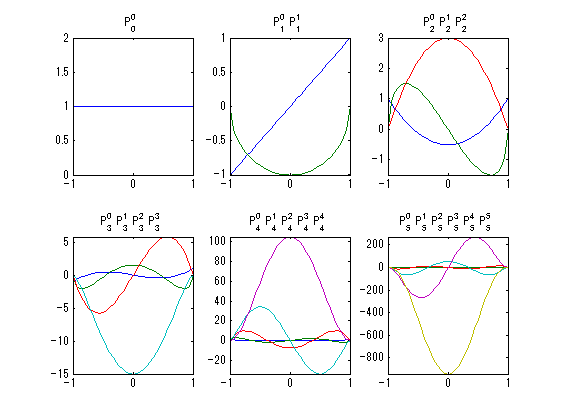
MATLABには幸いルジャンドル陪関数の関数legendreが用意してあります。 Pml=lengendre((l,~)とするとmの値を0~lに変化させた結果が返ってきます。 ルジャンドル陪関数は直交性があり、これを含む球面調和関数も直交性があります。
close all;clear;
seg=36;
x=linspace(-1,1,seg+1);
figure('color',[1,1,1],'InvertHardCopy','off');
P0l=[];
for m=0:6
    Pml=legendre(abs(m),x);
    P0l=[P0l;Pml(1,:)];
end;
plot(x,P0l);hold on;
L=legend('P_0^0','P_1^0','P_2^0','P_3^0','P_4^0','P_5^0','P_6^0');
set(L,'location','bestoutside');
axis tight;
title('Legendre function');
seg=36;
x=linspace(-1,1,seg+1);
figure('color',[1,1,1],'InvertHardCopy','off');
for l=0:5;
    subplot(2,3,l+1);
    Pml=legendre(l,x);
    plot(x,Pml);hold on;
    axis tight;
    st=[];
    for m=0:l
        st=[st,sprintf('P_%d^%d ',l,m)];
    end;
    title(st);
end;
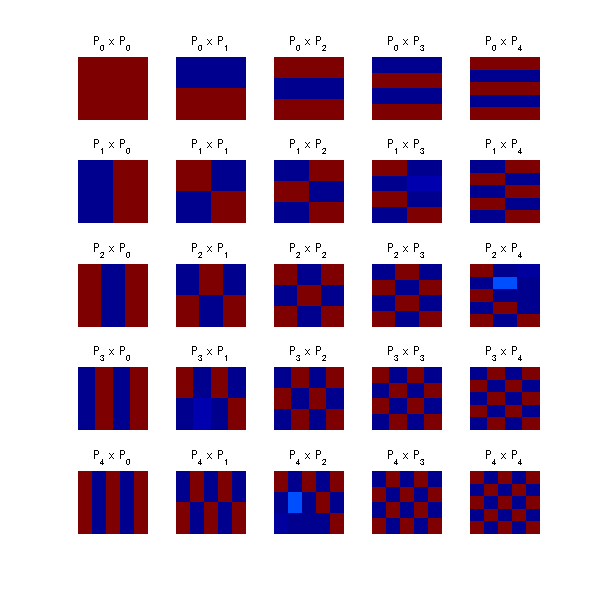
ルジャンドル陪関数の直交性の検討
m==m以外の時は内積はゼロになります。 式レベルで証明されています。 検討してみました。 青がゼロです。市松模様みたいになってしまいました。 丸めなどの計算誤差のせいなんだろうか?
close all;
figure('color',[1,1,1],'position',[50,50,600,600]);
seg=100;N=4;
t=linspace(-1,1,seg);
for x=0:N
    Px=legendre(x,t);
    for y=0:N
        K=legendre(y,t)*Px';
        subplot(N+1,N+1,x*(N+1)+y+1);
        imagesc(abs(K));
        title(sprintf('P_%d x P_%d',x,y));
        axis off;
    end;
end;
set(findobj(gcf,'type','axes'),'clim',[0,1]);
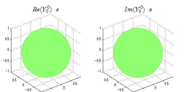
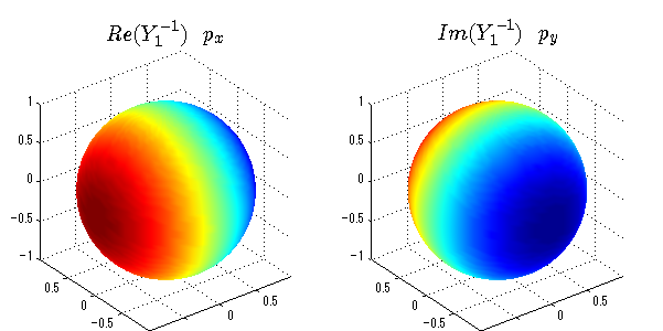
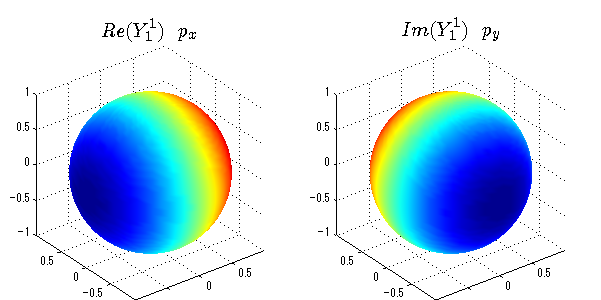
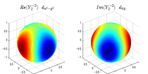
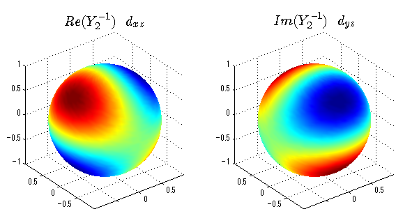
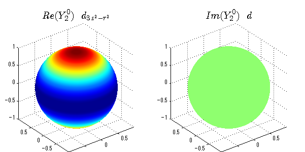
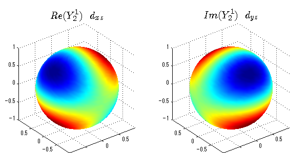
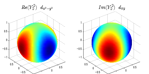
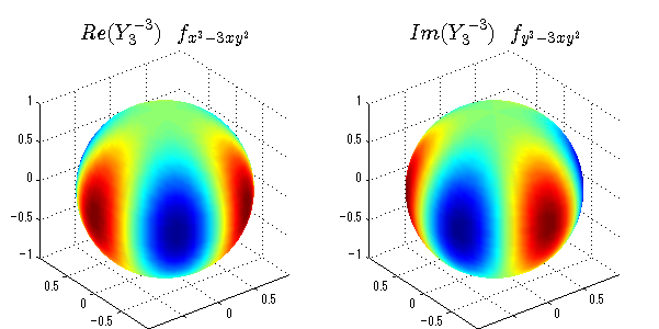
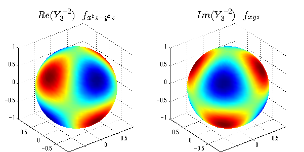
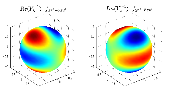
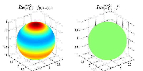
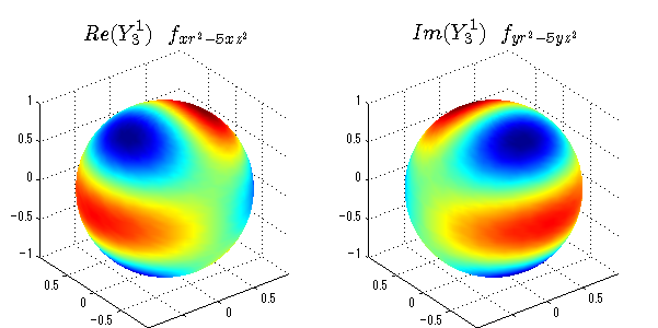
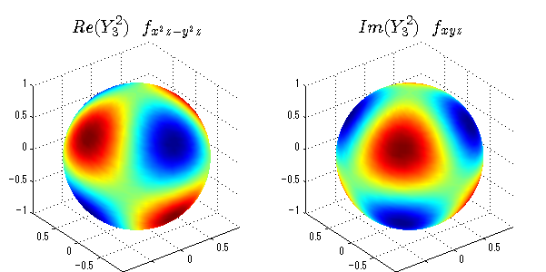
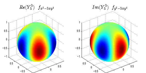
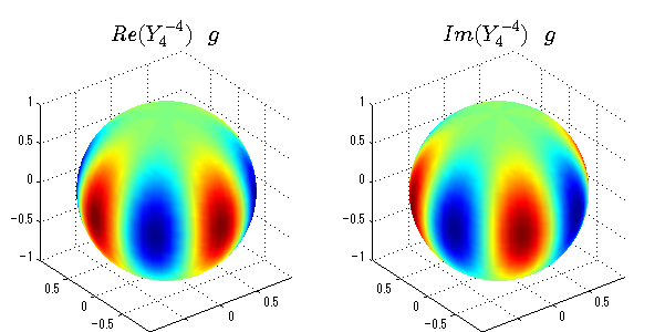
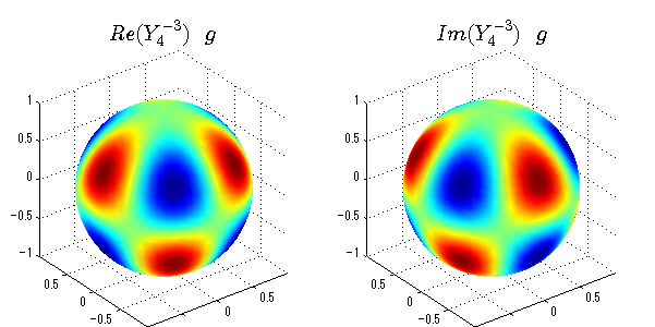
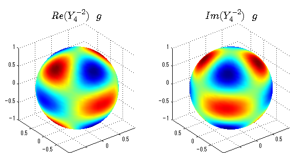
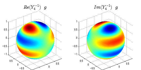
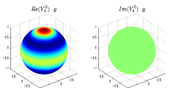
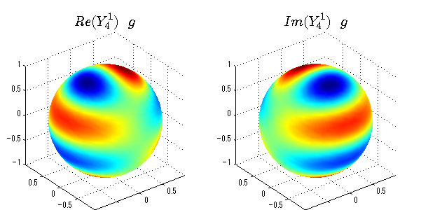
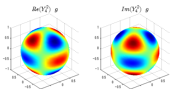
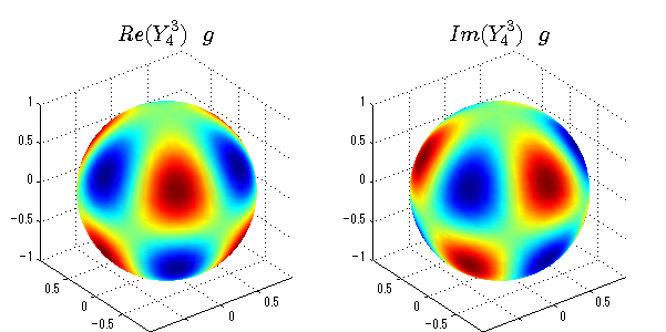
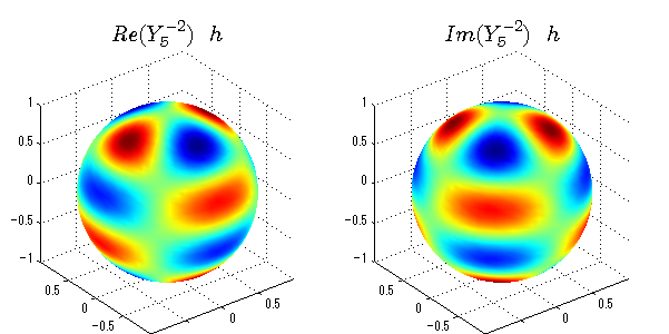
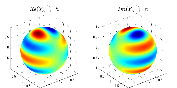
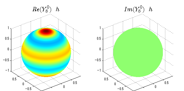
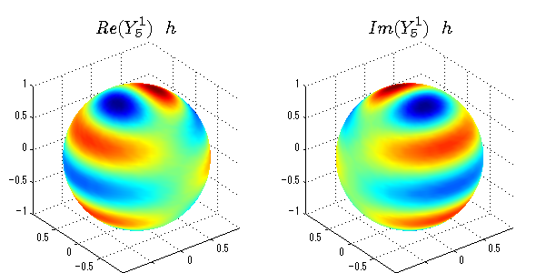
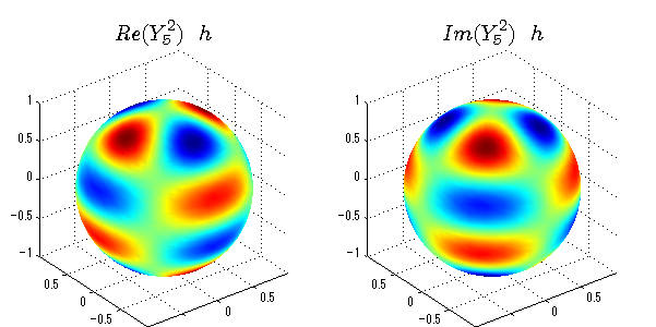
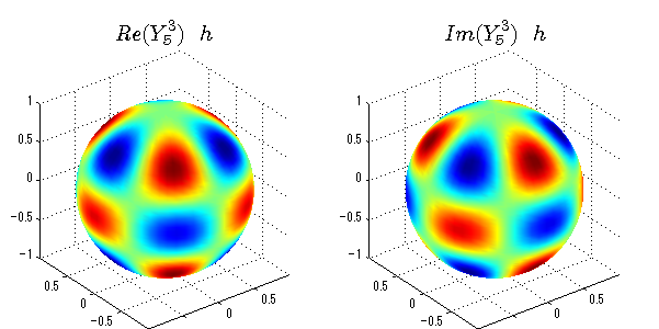
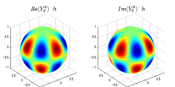
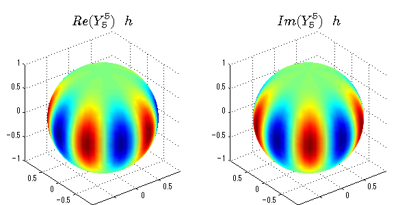
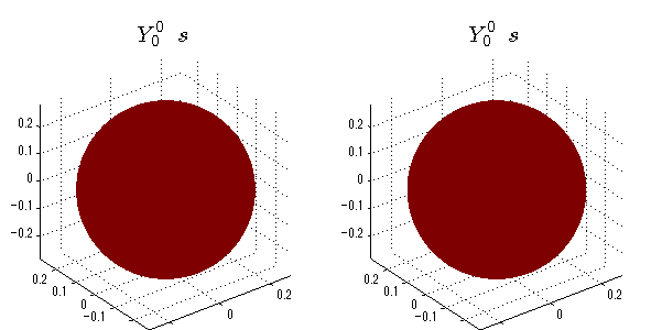
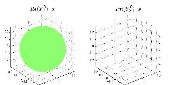
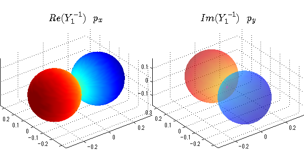
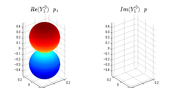
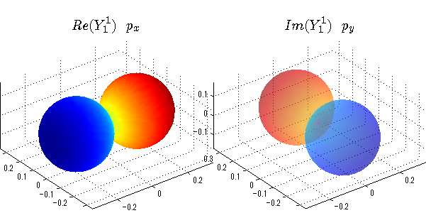
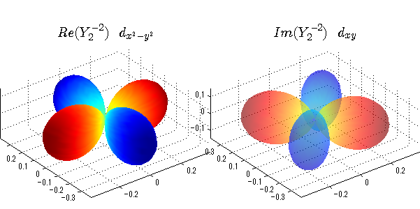
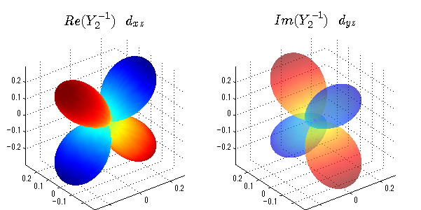
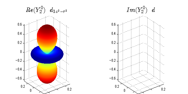
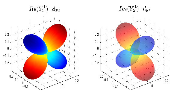
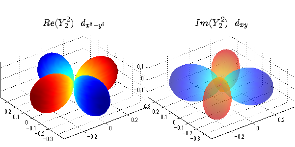
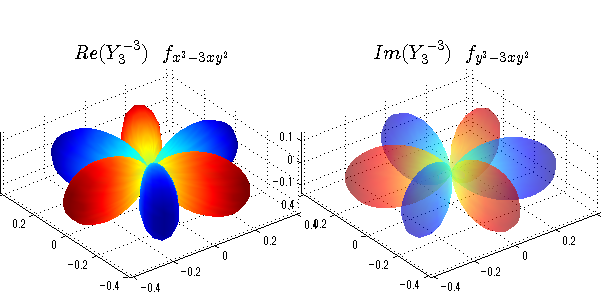
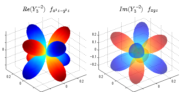
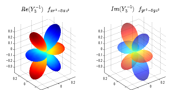
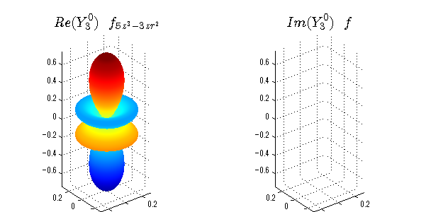
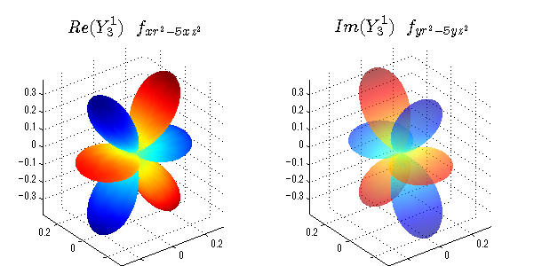
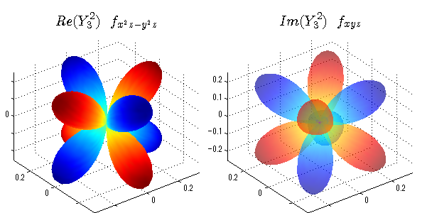
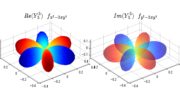
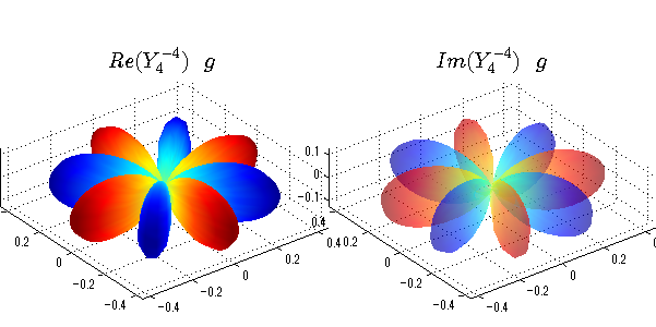
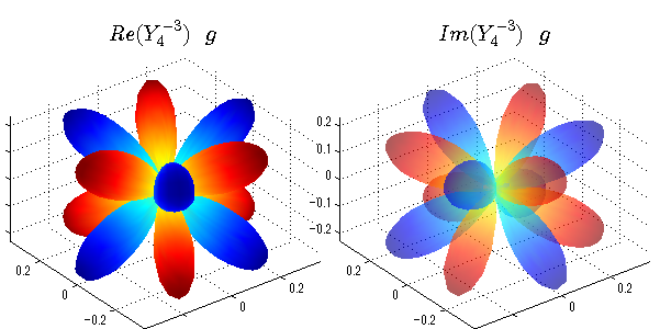
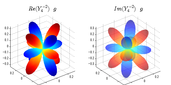
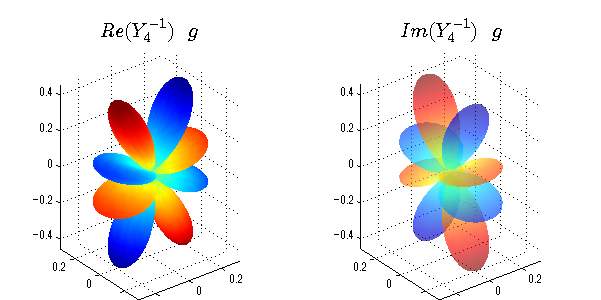
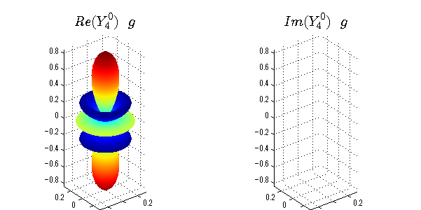
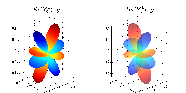
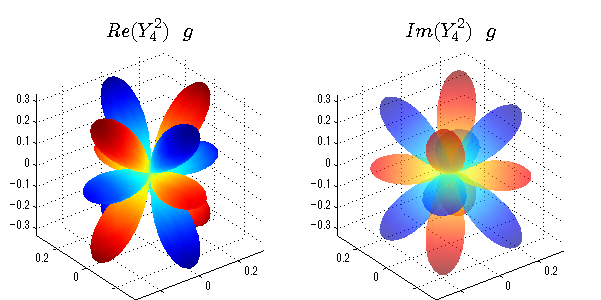
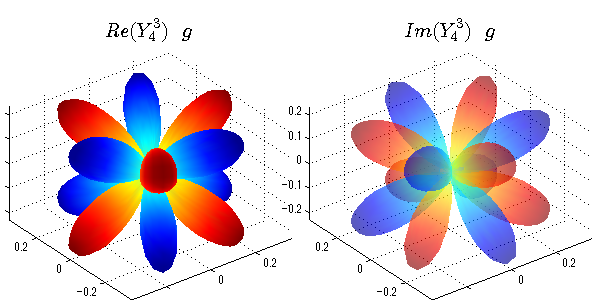
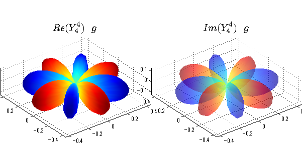
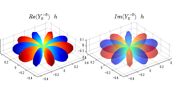
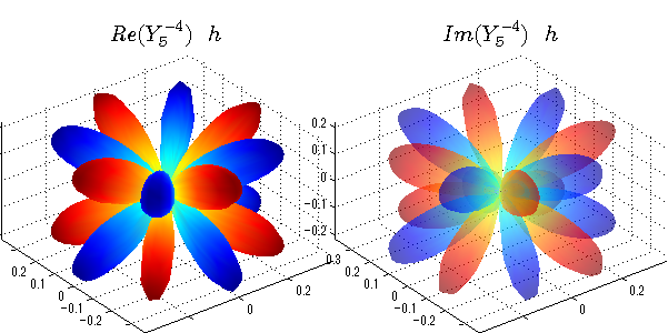
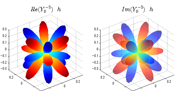
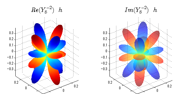
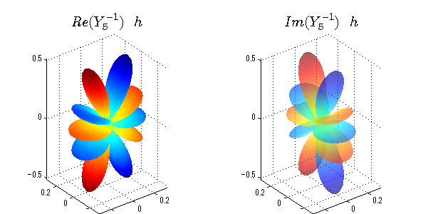
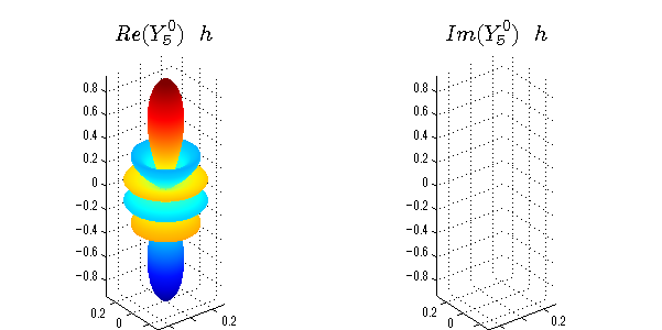
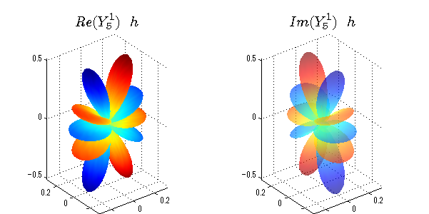
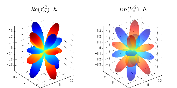
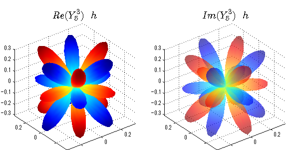
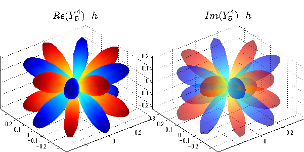
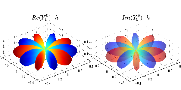
球面調和関数の作成 半径=1で実数・虚数別の球面表示
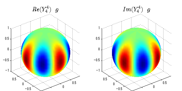
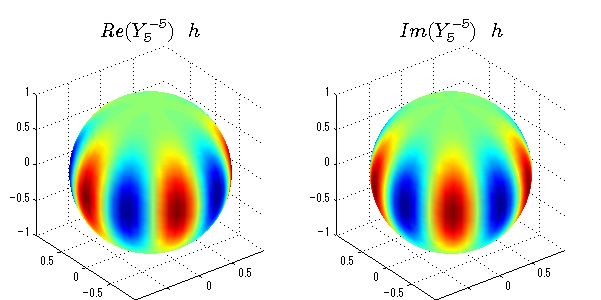
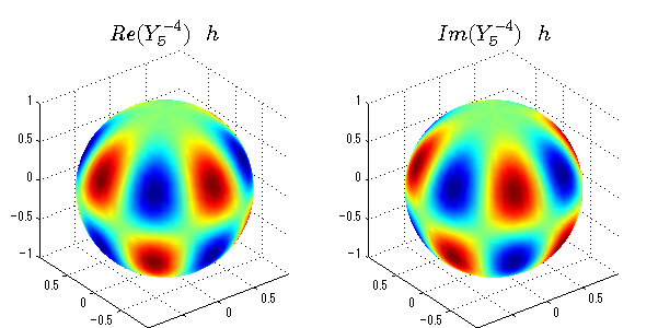
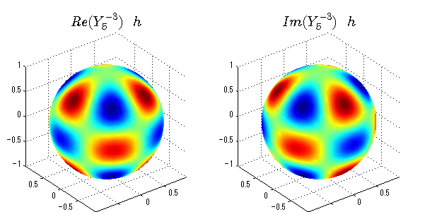
上記のlegendre関数を使って球面調和関数を作成できます。 Yの下段はl、上段はmです。lを0,1,2...と変化させてみました。 lにはs(harp),p(rinciple),d(iffuse),f(aint),g,h,i,・・・といった名前がついています。 本来複素表示なのですが、実数部分と虚数部分に分けて表示してみました。 zは軸方向、xは実数方向、yは虚数方向です。 中心からの距離=半径は1で統一しました。色は、実数部分、虚数部分の大きさを反映させました。 左が実数部分で、右が虚数部分です。m=0のとき、虚数部分はゼロとなります。 この図が一番わかりやすいと思います。要するにlは緯度方向の波の数、mは経度方向の波の数です。
close all;clear;
N=5;
seg=64;
theta=linspace(0,pi,seg);
phi=linspace(0,2*pi,seg);
Theta=theta'*ones(1,seg);
Phi=ones(seg,1)*phi;
x=sin(Theta).*cos(Phi);
y=sin(Theta).*sin(Phi);
z=cos(Theta);
for l=0:N;
    L=legendre(l,cos(theta));
    for m=-l:l;
        am=abs(m);
        LL=L(abs(m)+1,:);
        c=(-1)^((m+am)/2)*sqrt((2*l+1)/(4*pi)*factorial(l-am)/factorial(l+am))*LL'*exp(1i*m*phi);
        figure('color',[1,1,1],'inverthardcopy','off','position',[50,50,600,300]);

        for mm=1:2
            subplot('position',[(mm-1)*0.5,0,0.5,0.85]);
            if mm==1;cc=real(c);else cc=imag(c);end;
            h=surf(x,y,z,cc);
            set(h,'FaceColor','interp','EdgeColor','none');
            grid on;
            daspect([1,1,1]);
            axis tight;
            rotate3d on;

            if mm==1
                st1=sprintf('Re(Y_%d^{%d})',l,m);
            else
                st1=sprintf('Im(Y_%d^{%d})',l,m);
            end;
            switch l
                case 0;st2='s';st3='';
                case 1;
                    st2='p';
                    switch m;
                        case {-1,1};st3='_x';if mm==2;st3='_y';end;
                        case 0;st3='_z';     if mm==2;st3=''; end;
                    end;
                case 2;
                    st2='d_{';
                    switch m;
                        case {-2,2};st3='x^2-y^2}';if mm==2;st3='xy}';end;
                        case {-1,1};st3='xz}';     if mm==2;st3='yz}';end;
                        case  0;st3='3z^2-r^2}';   if mm==2;st3='}';end;
                    end;
                case 3;
                    st2='f_{';
                    switch m;
                        case {-3,3};st3='x^3-3xy^2}'; if mm==2;st3='y^3-3xy^2}';end;
                        case {-2,2};st3='x^2z-y^2z}'; if mm==2;st3='xyz}';end;
                        case {-1,1};st3='xr^2-5xz^2}';if mm==2;st3='yr^2-5yz^2}';end;
                        case  0;st3='5z^3-3zr^2}';    if mm==2;st3='}';end;
                    end;
                case 4;st2='g';st3='';
                case 5;st2='h';st3='';
            end;
            title(['$$',st1,'\ \ ',st2,st3,'$$'],'interpreter','latex','FontSize',15);
        end;

    end;
end;

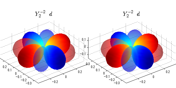
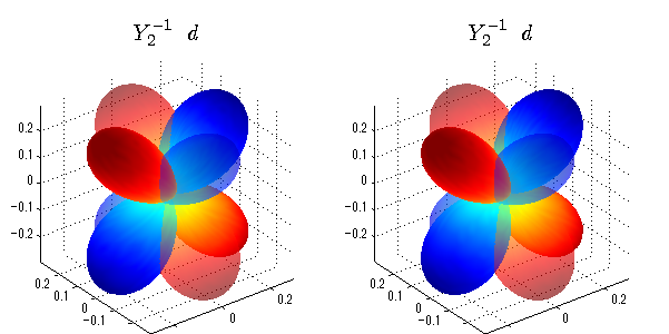
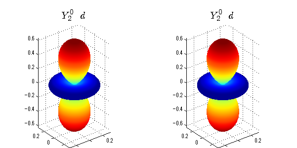
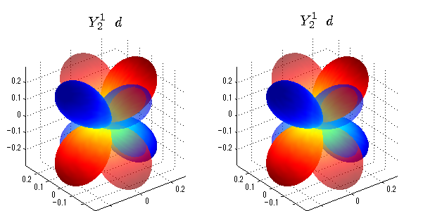
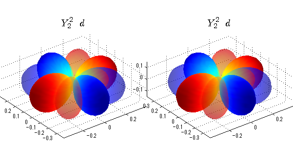
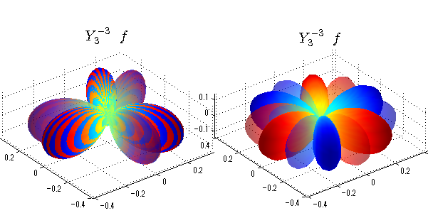
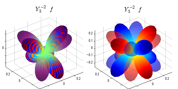
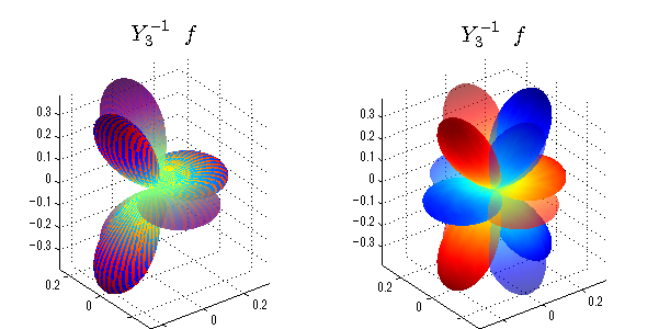
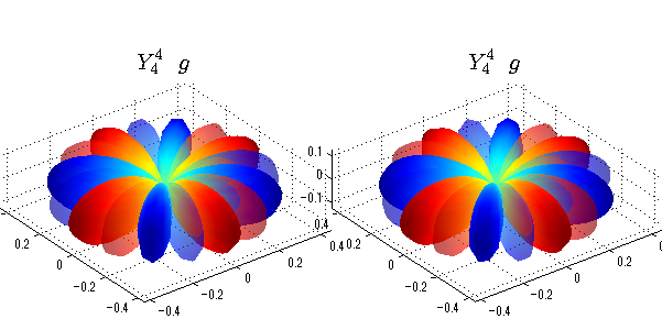
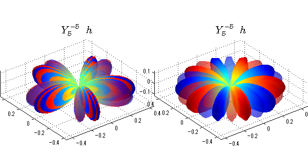
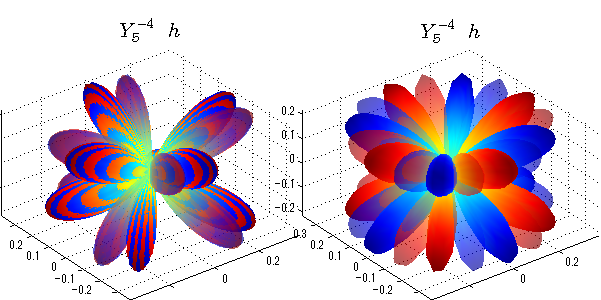
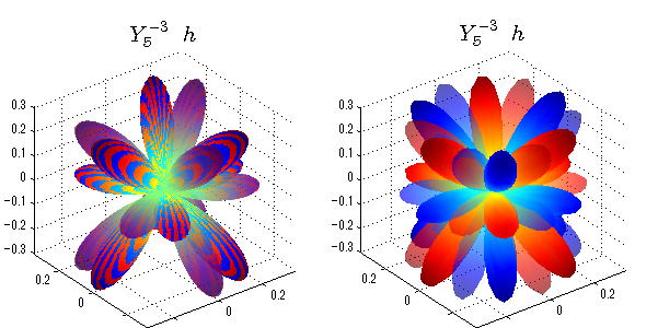
球面調和関数 半径の正負/絶対値表示
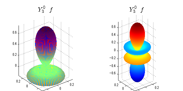
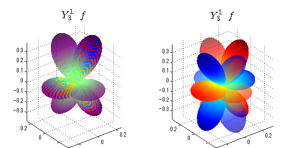
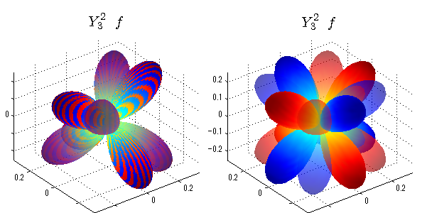
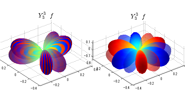
中心からの距離は実数・虚数の値を反映させました。 左図はマイナスの距離を含むそのままの値を、 右図はた時の絶対値で表しています。 色は実数・虚数部分の大きさを反映させました。 虚数部分は半透明にしてます。 中心からの距離を絶対値表示しないとlが奇数の時は、実数部分がマイナスの距離になり、表面が重なって縞々になります。
close all;clear;
N=5;
seg=64;
theta=linspace(0,pi,seg);
phi=linspace(0,2*pi,seg);
Theta=theta'*ones(1,seg);
Phi=ones(seg,1)*phi;
x=sin(Theta).*cos(Phi);
y=sin(Theta).*sin(Phi);
z=cos(Theta);
for l=0:N;
    L=legendre(l,cos(theta));
    for m=-l:l;
        am=abs(m);
        LL=L(abs(m)+1,:);
        c=(-1)^((m+am)/2)*sqrt((2*l+1)/(4*pi)*factorial(l-am)/factorial(l+am))*LL'*exp(1i*m*phi);
        figure('color',[1,1,1],'inverthardcopy','off','position',[50,50,600,300]);

        for mm=1:2
            subplot('position',[(mm-1)*0.5,0,0.5,0.85]);
            cc=real(c);
            if mm==1;r=cc;else r=abs(cc);end;
            h=surf(r.*x,r.*y,r.*z,cc);hold on;
            set(h,'FaceColor','interp','EdgeColor','none');
            cc=imag(c);
            if mm==1;r=cc;else r=abs(cc);end;
            h=surf(r.*x,r.*y,r.*z,cc);hold on;
            set(h,'FaceColor','interp','EdgeColor','none','FaceAlpha',0.4);

            grid on;
            daspect([1,1,1]);
            axis tight;
            rotate3d on;
            st1=sprintf('Y_%d^{%d}',l,m);
            switch l
                case 0;st2='s';
                case 1;st2='p';
                case 2;st2='d';
                case 3;st2='f';
                case 4;st2='g';
                case 5;st2='h';
            end;
            title(['$$',st1,'\ \ ',st2,'$$'],'interpreter','latex','FontSize',15);
        end;

    end;
end;
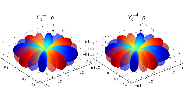
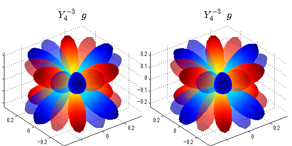
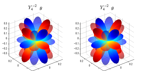
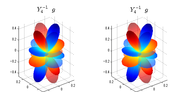
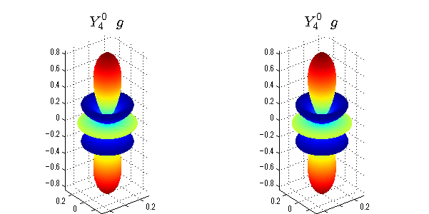
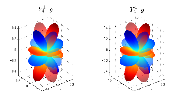
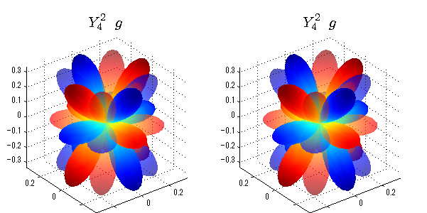
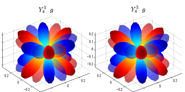
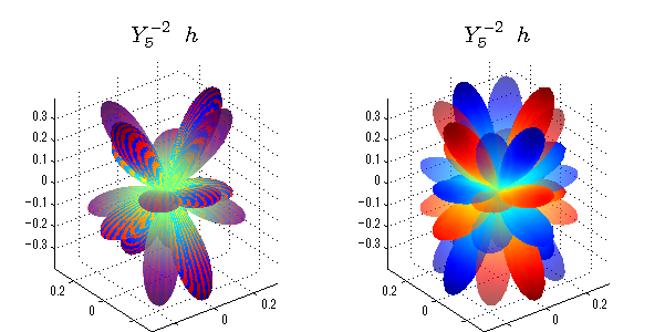
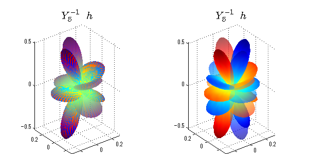
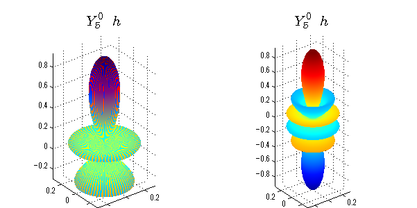
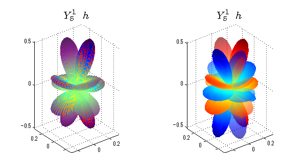
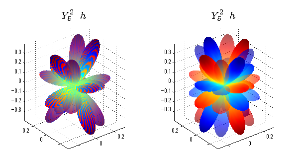
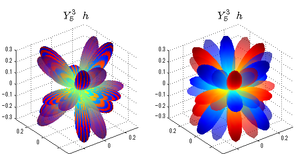
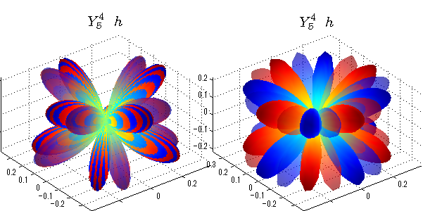
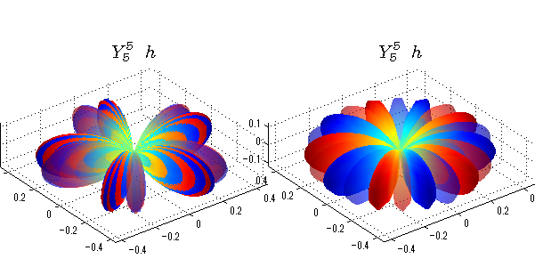
球面調和関数 実数・虚数別表示
実数と虚数に分けて表示させました。 左は実数部分、右は虚数部分です。虚数部分は半透明としました。 中心からの距離を実数・虚数の値の絶対値で反映させました。 色はマイナスが赤で、プラスが青です。
close all;clear;
N=5;
seg=64;
theta=linspace(0,pi,seg);
phi=linspace(0,2*pi,seg);
Theta=theta'*ones(1,seg);
Phi=ones(seg,1)*phi;
x=sin(Theta).*cos(Phi);
y=sin(Theta).*sin(Phi);
z=cos(Theta);
for l=0:N
    L=legendre(l,cos(theta));
    for m=-l:l;
        am=abs(m);
        LL=L(abs(m)+1,:);
        c=(-1)^((m+am)/2)*sqrt((2*l+1)/(4*pi)*factorial(l-am)/factorial(l+am))*LL'*exp(1i*m*phi);
        figure('color',[1,1,1],'inverthardcopy','off','position',[50,50,600,300]);

        for mm=1:2
            cc=abs(c);
            cx=cc.*x;cy=cc.*y;cz=cc.*z;
            cx=[min(cx(:)),max(cx(:))];
            cy=[min(cy(:)),max(cy(:))];
            cz=[min(cz(:)),max(cz(:))];
            if mm==1;
                cc=real(c);r=abs(cc);
            else
                cc=imag(c);r=abs(cc);
            end;
            subplot('position',[(mm-1)*0.5,0,0.5,0.85]);
            h=surf(r.*x,r.*y,r.*z,cc);hold on;
            set(h,'FaceColor','interp','EdgeColor','none');
            if mm==2;set(h,'FaceAlpha',0.4);end;
            grid on;
            daspect([1,1,1]);
            set(gca,'xlim',cx,'ylim',cy,'zlim',cz);
            % axis tight;
            rotate3d on;
            st1=sprintf('Y_%d^{%d}',l,m);
            if mm==1
                st1=sprintf('Re(Y_%d^{%d})',l,m);
            else
                st1=sprintf('Im(Y_%d^{%d})',l,m);
            end;
            switch l
                case 0;st2='s';st3='';
                case 1;
                    st2='p';
                    switch m;
                        case {-1,1};st3='_x';if mm==2;st3='_y';end;
                        case 0;st3='_z';     if mm==2;st3=''; end;
                    end;
                case 2;
                    st2='d_{';
                    switch m;
                        case {-2,2};st3='x^2-y^2}';if mm==2;st3='xy}';end;
                        case {-1,1};st3='xz}';     if mm==2;st3='yz}';end;
                        case  0;st3='3z^2-r^2}';   if mm==2;st3='}';end;
                    end;
                case 3;
                    st2='f_{';
                    switch m;
                        case {-3,3};st3='x^3-3xy^2}'; if mm==2;st3='y^3-3xy^2}';end;
                        case {-2,2};st3='x^2z-y^2z}'; if mm==2;st3='xyz}';end;
                        case {-1,1};st3='xr^2-5xz^2}';if mm==2;st3='yr^2-5yz^2}';end;
                        case  0;st3='5z^3-3zr^2}';    if mm==2;st3='}';end;
                    end;
                case 4;st2='g';st3='';
                case 5;st2='h';st3='';
            end;

            title(['$$',st1,'\ \ ',st2,st3,'$$'],'interpreter','latex','FontSize',15);
        end;
    end;
end;
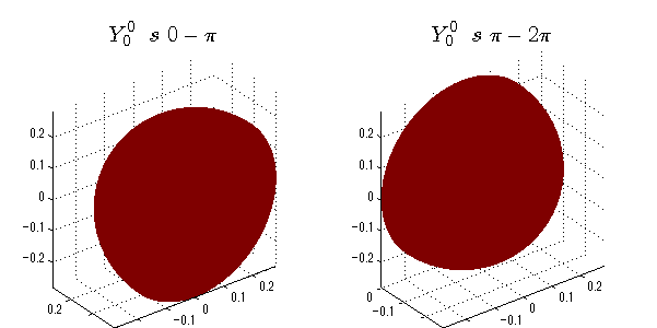
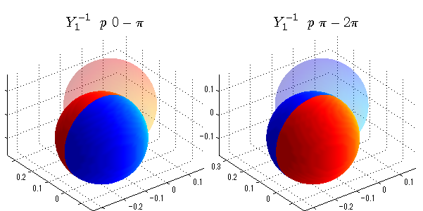
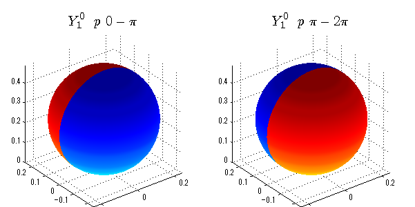
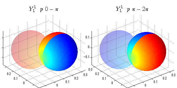
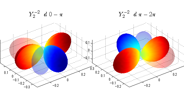
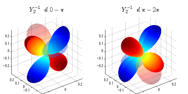
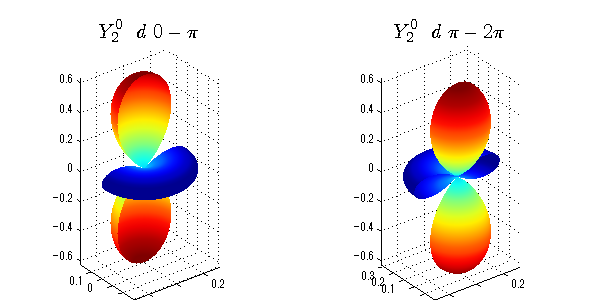
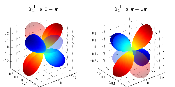
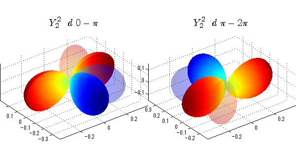
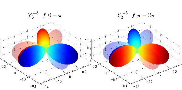
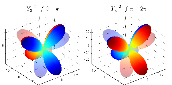
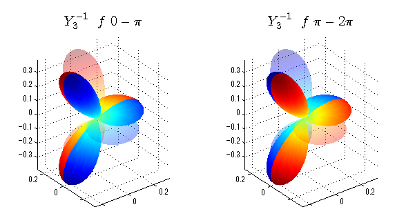
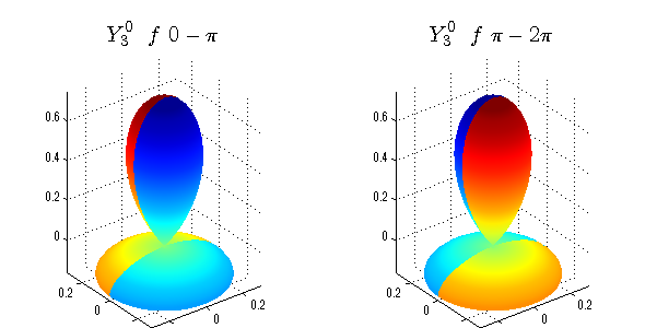
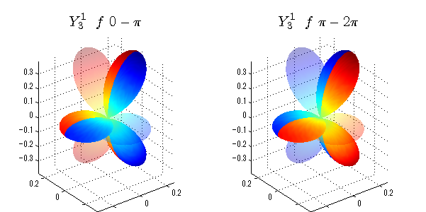
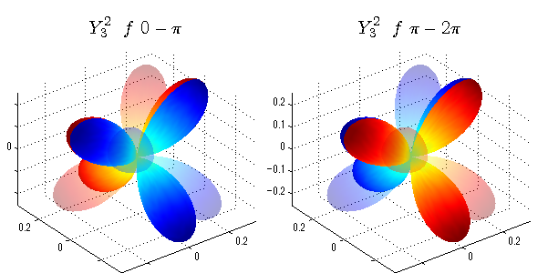
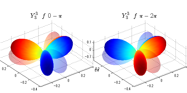
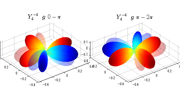
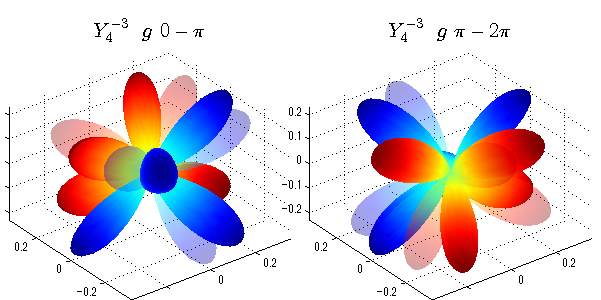
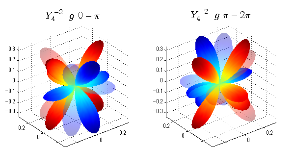
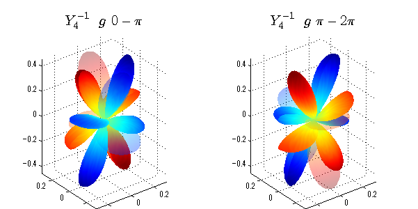
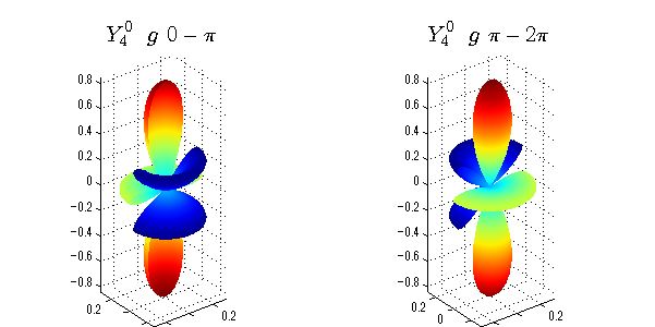
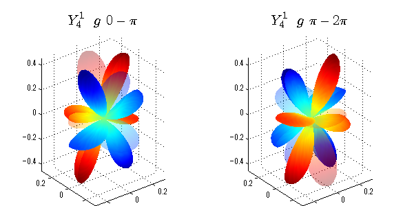
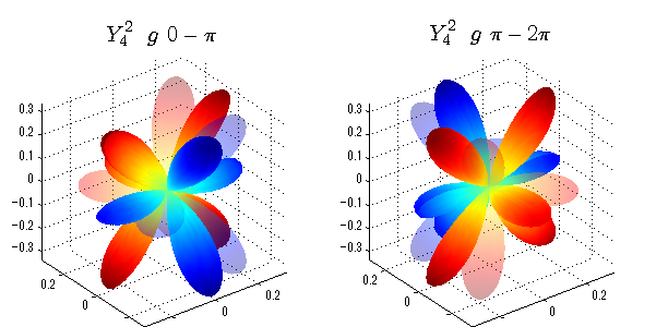
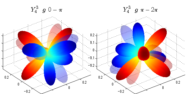
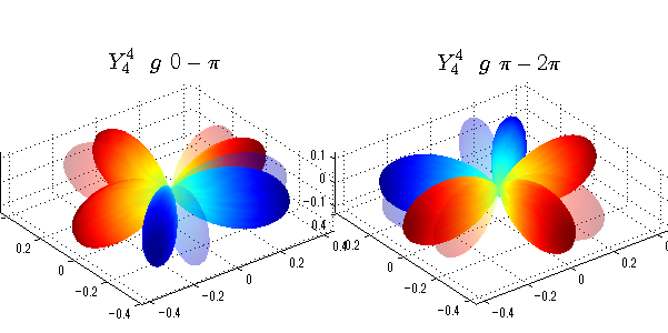
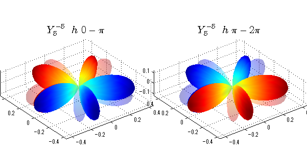
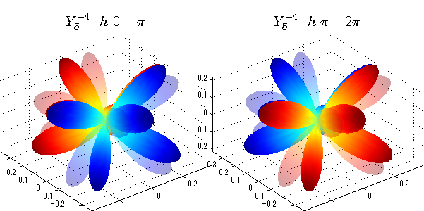
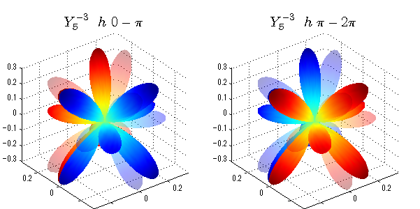
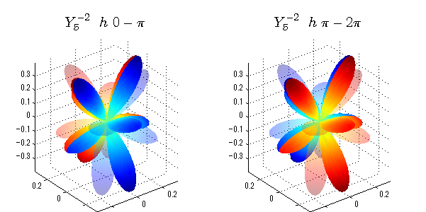
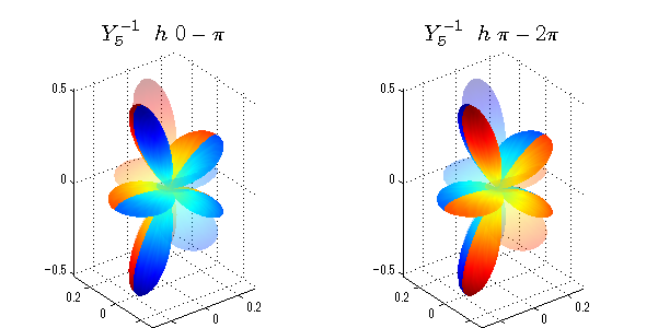
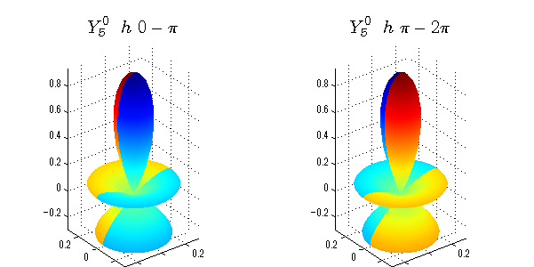
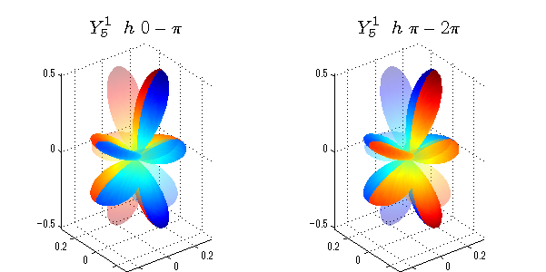
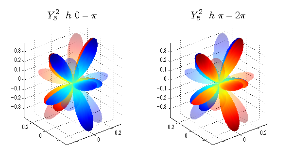
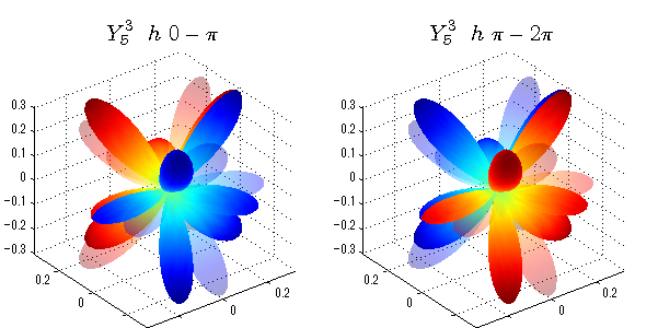
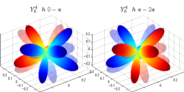
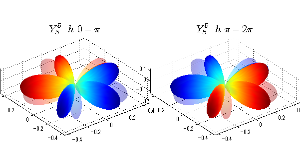
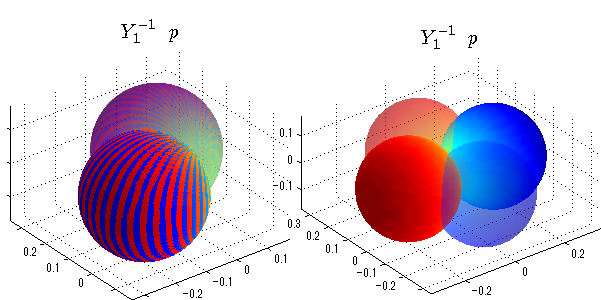
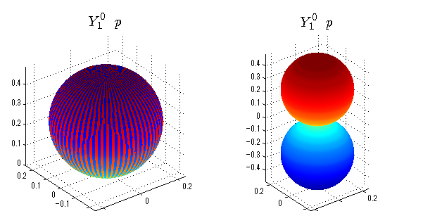
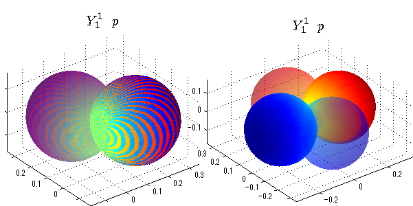
球面調和関数 位相別表示
phiを0~π、π~2πにわけて絶対値でなく、そのまま表示としました。
close all;clear;
N=5;
seg=64;
theta=linspace(0,pi,seg);
phi1=linspace(0,pi,seg);
phi2=linspace(pi,2*pi,seg);
Theta=theta'*ones(1,seg);
Phi1=ones(seg,1)*phi1;
Phi2=ones(seg,1)*phi2;
x1=sin(Theta).*cos(Phi1);
y1=sin(Theta).*sin(Phi1);
x2=sin(Theta).*cos(Phi2);
y2=sin(Theta).*sin(Phi2);
z=cos(Theta);
for l=0:N;
    L=legendre(l,cos(theta));
    for m=-l:l;
        am=abs(m);
        LL=L(abs(m)+1,:);
        figure('color',[1,1,1],'inverthardcopy','off','position',[50,50,600,300]);
        for mm=1:2
            switch mm
                case 1;phi=phi1;x=x1;y=y1;
                case 2;phi=phi2;x=x2;y=y2;
            end;
            c=(-1)^((m+am)/2)*sqrt((2*l+1)/(4*pi)*factorial(l-am)/factorial(l+am))*LL'*exp(1i*m*phi);
            subplot('position',[(mm-1)*0.5,0,0.5,0.85]);
            cc=real(c);r=cc;
            h=surf(r.*x,r.*y,r.*z,cc);hold on;
            set(h,'FaceColor','interp','EdgeColor','none');
            cc=imag(c);r=cc;
            h=surf(r.*x,r.*y,r.*z,cc);hold on;
            set(h,'FaceColor','interp','EdgeColor','none','FaceAlpha',0.2);

            grid on;
            daspect([1,1,1]);
            axis tight;
            rotate3d on;
            st1=sprintf('Y_%d^{%d}',l,m);
            switch l
                case 0;st2='s';
                case 1;st2='p';
                case 2;st2='d';
                case 3;st2='f';
                case 4;st2='g';
                case 5;st2='h';
            end;
            if mm==1;st3='\ 0-\pi';else st3='\ \pi-2\pi';end;
            title(['$$',st1,'\ \ ',st2,st3,'$$'],'interpreter','latex','FontSize',15);
        end;

    end;
end;